Reinforcement Learning: An Introduction With Python Examples

Basic and deep reinforcement learning (RL) models can often resemble science-fiction AI more than any large language model today. Let’s take a look at how RL enables this agent to complete a very difficult level in Super Mario:

At first, the agent has no idea how to play this game. It doesn’t know the controls, how to make progress, what the obstacles are, or what finishes the game. The agent must learn all these things without any human intervention—all through the power of reinforcement learning algorithms.

RL agents can solve problems without predefined solutions or explicitly programmed actions and most importantly, without large amounts of data. That’s why RL is having a significant impact on many fields. For instance, it’s used in:

• Self-driving cars: RL agents can learn optimal driving strategies based on traffic conditions and road rules.
• Robotics: Robots can be trained to perform complex tasks in dynamic environments through RL.
• Game playing: AI agents can learn complex strategies in games like Go or StarCraft II using RL techniques.

Reinforcement learning is a rapidly evolving field with vast potential. As research progresses, we can expect even more groundbreaking applications in areas like resource management, healthcare, and personalized learning.

That’s why now is a great time to learn about this fascinating field of machine learning. In this tutorial, we’ll help you understand the fundamentals of reinforcement learning and explain step-by-step concepts like agent, environment, action, state, rewards, and more.

Agent and Environment

Let’s say you want to teach your cat, Bob, how to use multiple scratching posts in a room instead of your expensive furniture. In reinforcement learning terms, Bob is the agent, the learner, and the decision maker. It needs to learn which things are okay to scratch (rugs and posts) and which are not (couches and drapes).

The room is called the environment with which our agent interacts. It provides challenges (tempting furniture) and the desired objective (a satisfying scratching post).

There are two main types of environments in RL:

• Discrete environments: If the room turned into a classic arcade game with a grid, Bob could only move in four directions. Such environments have a limited number of options for both Bob’s actions and the variations of the room.
• Continuous environments: A real-world room allows nearly infinite possibilities to arrange the scratching posts and furniture. Besides, Bob is free to do anything cats usually do every day. That’s why our room is a continuous environment with endless possibilities for Bob and the room.

Our room is also a static environment. The furniture doesn’t move, and the scratching posts stay put.

But if you randomly move around the furniture and scratching posts once every few hours (like different levels of the Super Mario game), the room would become a dynamic environment, which is trickier for an agent to learn because things keep changing.

Actions and States

Two important aspects of all reinforcement learning problems are state space and action space.

State space represents all possible states (situations) in which the agent and the environment find themselves at any given moment. The size of the state space depends on the environment type:

• Finite state space: When the environment is discrete, the number of possible states is finite or countably infinite. Examples are board games, grid-like video games, or tic-tac-toe.
• Infinite state space: When the environment is continuous, its state space is unbounded. Examples are video games with complex characters and environments, robots learning to walk, or in our case, cats learning to use a scratching post.

The action space is all the things Bob can do in the environment. In our scratching post example, Bob’s actions could be scratching the post, napping on the couch, or even chasing its tail.

Similar to the state space, the number of actions Bob can take depends on the environment:

• Discrete Environments: In a grid-world game, Bob might have a limited number of actions, like moving up, down, left, or right and scratching.
• Continuous Environments: In a real-world room, Bob might have a broader range of actions, like moving in any direction, jumping, or even (hopefully not) chewing on wires.

When Bob starts his scratching post adventure, the environment is in a default state, let’s call it state zero. In our case, this might be the room with the scratching post set up. Every action it takes moves the environment into new subsequent states.

Rewards, Time Steps, and Episodes

For Bob to achieve its overall goal, it needs incentives or rewards.

Most RL problems have pre-defined rewards. For example, in chess, capturing a piece is a positive reward, while receiving a check is a negative reward.

In our case, we may give Bob treats if we observe a positive action, such as not scratching furniture for some time or if it actually finds one of the scratching posts. We might also punish it with some water squirts in the face if it claws up drapes.

To measure Bob’s learning journey's progress, we can think of its actions in terms of time steps. For instance, at time step t₁, Bob takes action a₁, which results in a new state s₁ (s₀ was the default state). It may also receive a reward r₁.

A collection of time steps is called an episode. An episode always starts in a default state (the furniture and posts are set up) and terminates when the objective is reached (a post is found) or the agent fails (scratches furniture). Sometimes, an episode may also terminate based on how much time has passed (like in chess).

Exploration vs. Exploitation

Like a skilled chess player, Bob shouldn’t just seek any scratching post. Bob should want the one that yields the most rewarding treats. This highlights a classical dilemma in reinforcement learning: exploration vs. exploitation.

While a tempting post might offer immediate gratification, a more strategic exploration could lead to a jackpot treat later. Just as a chess player might forgo a capture to gain a superior position, Bob might initially scratch a suboptimal post (exploration) to discover the ultimate scratching haven (exploitation). This long-term strategy is crucial for agents to maximize rewards in complex environments.

In other words, Bob must balance exploitation (sticking to what works best) with exploration (occasionally venturing out to look for new scratching posts). Exploring too much might waste time, especially in continuous environments, while exploiting too much might make Bob miss out on something even better.

Luckily, there are some clever strategies Bob can take:

• Epsilon-greedy learning: Let’s imagine for a second that Bob has a special “scratchy-meter” that generates random numbers. If the generated number is smaller than some predefined threshold called epsilon, Bob tries a random scratching surface (exploration). But if the number is greater than epsilon, Bob goes for the post that felt best before (exploitation).
• Boltzmann exploration: If Bob keeps scratching things that don't feel right (getting negative rewards), it's more likely to explore new options (increased exploration). But as he finds the perfect scratching post (positive rewards), he'll stick to that happy spot (exploitation).

By using these strategies (or others that fall beyond the scope of our tutorial), Bob can find a balance between exploring the unknown and sticking to the good stuff.

Reinforcement Learning Algorithms

Bob can’t figure out how to maximize the number of treats all by itself. It needs some methods and tools to guide its decisions in every state of the environment. This is where reinforcement learning algorithms come to Bob’s rescue.

From a broader perspective, reinforcement learning algorithms can be categorized based on how they make agents interact with the environment and learn from experience. The two main categories of reinforcement learning algorithms are model-based and model-free.

Model-based reinforcement learning

In model-based algorithms, the agent (like Bob) builds an internal model of the environment. This model represents the dynamics of the environment, including state transitions and reward probabilities. The agent can then use this model to plan and evaluate different actions before taking them in the real environment.

This approach has the advantage of being more sample-efficient, especially in complex environments. This means Bob might require fewer scratching attempts to identify the optimal post compared to purely trial-and-error approaches. And that’s because Bob can plan and evaluate before taking action.

The disadvantage is that building an accurate model can be challenging, especially for complex environments. The model may not accurately reflect the real environment, leading to suboptimal behavior.

A common model-based RL algorithm is Dyna-Q, which actually combines model-based and model-free learning. It constructs a model of the environment and utilizes it for action planning while simultaneously learning directly from experience through model-free Q-learning (which we'll explain in a bit).

Model-free reinforcement learning

This approach focuses on learning directly from interaction with the environment without explicitly building an internal model. The agent (Bob) learns the value of states and actions or the optimal strategy through trial and error.

Model-free RL offers a simpler approach in environments where building an accurate model is challenging. For Bob, this means he doesn't need to create a complex mental map of the room – he can learn through scratching and experiencing the consequences.

Model-free RL excels in dynamic environments where the rules might change. If the room's furniture layout changes, Bob can adapt his exploration and learn the new optimal scratching spots.

However, only learning through trial and error can be less sample-efficient. Bob might need to scratch a lot of furniture before consistently finding the most rewarding post.

Some common model-free RL algorithms include:

• Q-Learning: The algorithm learns a Q-value for each state-action pair. The Q-value represents the expected future reward of taking a specific action in a particular state. The agent can then choose the action with the highest Q-value to maximize its long-term reward (we’ll explain this in more detail in the next section).
• SARSA (State-Action-Reward-State-Action): This is similar to Q-learning, but it learns a value function for each state-action pair. It updates the value based on the reward received after taking an action and the next state observed.
• Policy gradient methods: These algorithms directly learn the policy function, which maps states to actions. They use gradients to update the policy in the direction expected to lead to higher rewards. Examples include REINFORCE and Proximal Policy Optimization (PPO).
• Deep Q-Networks (DQN): This algorithm combines Q-learning with deep neural networks to handle high-dimensional state spaces, often encountered in complex environments like video games.

What algorithm we should choose depends on various factors: the complexity of the environment, the availability of resources, or the desired level of interpretability.

Model-based approaches might be preferable for simpler environments where building an accurate model is feasible. On the other hand, model-free approaches are often more practical for complex, real-world scenarios.

Additionally, with the rise of deep learning, Deep Q-Networks (DQN) and other deep RL algorithms are becoming increasingly popular for tackling complex tasks with high-dimensional state spaces.

Q-learning

Let’s now focus on a single algorithm and learn more about Q-learning.

High-level overview

Q-learning is a model-free algorithm that teaches agents the optimal winning strategy through smart interactions with the environment.

Let’s return to our cat example and imagine we’re solving an arcade version of the problem with a discrete environment and a finite set of actions.

Let’s say we give Bob a table. The columns represent the available actions, while each row maps the action to a specific state from the state space.

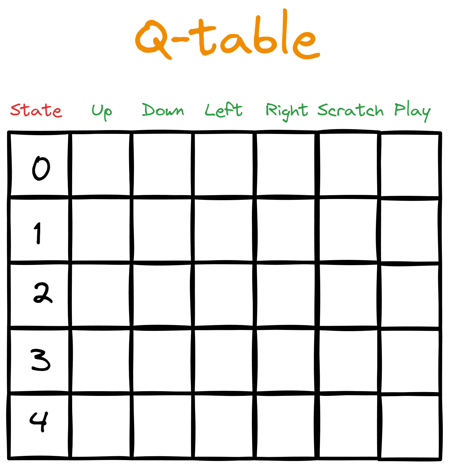
At first, we fill the table with zeros, representing the initial Q-values—for this reason, we call this a Q-table.

Then, we start an interaction loop from the default state (the start of an episode). In the loop, Bob takes the action with the highest Q-value for the given state. However, on the first pass through the loop, there won't be any highest Q-value to guide Bob's action since all Q-values are initially zero.

This is where exploration strategies (like random exploration or epsilon-greedy) come into play. These strategies help Bob gather information when the Q-table is empty.

Once the Q-table has been updated, Bob starts an interaction loop again. The action it takes results in a reward and a new state. Then, we calculate new Q-values for each action Bob can take in the new state (we’ll show in a bit how to calculate Q-values).

The episode continues until termination (Bob can take any number of steps in each episode), and then we start again. Each subsequent episode will have a richer Q-table, making Bob smarter.

Here is a high-level overview of the steps involved:

1. We initialize a Q-table and fill it with initial values.
2. We start an episode.
3. The agent takes action.
4. We measure the reward received.
5. A new state is reached.
6. A new Q-value is calculated for the new state.
7. The episode terminates either from failure or win or time-out.
8. The environment is reset.
9. We repeat steps 2-8 for the desired number of episodes.

Steps like one and two might be straightforward, but the rest need more explanation.

How does the agent choose the action?

At time step 1, when Bob takes his first action, it’ll be random, since all Q-values are zero. In subsequent time steps, Bob has to consider the balance between exploration and exploitation.

To help with that, we give Bob a hyperparameter called epsilon with a small value—typically 0.1. Then, we tell Bob to generate a random number between 0 and 1 and if the number is smaller than epsilon, he will choose a random action regardless of its Q-value.

If it’s higher than epsilon, Bob will choose the action with the highest Q-value. This way, Bob will be exploring epsilon (0.1 or 10%) of the time and exploiting (1 - epsilon or 0.9 or 90%) of the time.

What we just described is called the epsilon-greedy policy. Policies define how the agent takes action and how the Q-values are calculated.

How is the reward measured?

The rules for calculating the reward are usually set by the person who creates the environment. For example, you might decide to give Bob a single treat for using a scratch rug and five treats for jumping high enough to scratch the one on the wall. There’s also a chance you might punish Bob for scratching valuable objects.

But most of the time, there will be no reward since Bob will either sleep, walk, or play.

How do we update the Q-table?

The formula for calculating the Q-value can be intimidating, so let’s see it first in full length and then explain it step-by-step:

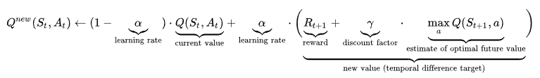
Let’s consider the beginning of the formula:

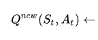
This part says, “Given the previous state and action, the new Q-value is calculated as (...).”

The part below is the current Q-value (soon-to-be old) the agent used to do the action.

Now let’s consider the final part:

S_t+1 is the new state resulting from taking action A_t. So, this part is finding the largest Q-value from all actions (a) in that new state. We multiply that value by a parameter γ called gamma (discount factor) and add the result to the reward received.

If we set gamma close to 1, we put a heavier weight on future rewards. If we dial it down towards zero, we emphasize the current reward R_t+1 more. This means gamma is another parameter we can use to balance exploration and exploitation.

Finally, we have alpha (α), which controls the training speed and ranges from 0 to 1. Values close to 1 make Q-values updates larger, so the agent learns quicker, making the right side of the plus sign heavier. In contrast, values close to 0 make the left side heavier, which contains the current Q-value.

Using the learning rate to control training speed ensures the agent doesn’t progress too quickly and forgets old information. It also ensures it doesn’t learn very slowly, possibly missing out on important information.

This is the most challenging part of understanding Q-learning, and I hope you got a rough feel for how it works.

Reinforcement Learning in Python Gymnasium

As with anything, Python has frameworks for solving reinforcement learning problems. The most popular one is Gymnasium, which comes pre-built with over 2000 environments (all documented thoroughly).

$ pip install "gymnasium[atari]"
$ pip install autorom[accept-rom-license]
$ AutoROM --accept-license

import gymnasium as gym
env = gym.make("ALE/Breakout-v5")

The environment we just loaded is called Breakout. Here is what it looks like:

The objective here is for the board (the agent) to learn how to eliminate all the bricks through trial and error. The rules of the game dictate the penalties and rewards.

We’ll finish the article by showing how you can run your own interaction episodes and visualize the agent’s progress with a GIF like the one above.

Here is the code for the interaction loop:

epochs = 0

frames = []  # for animation
done = False

env = gym.make("ALE/Breakout-v5", render_mode="rgb_array")
observation, info = env.reset()

while not done:
    action = env.action_space.sample()
    observation, reward, terminated, truncated, info = env.step(action)

    # Put each rendered frame into dict for animation
    frames.append(
        {
            "frame": env.render(),
            "state": observation,
            "action": action,
            "reward": reward,
        }
    )

    epochs += 1
    if epochs == 1000:
        break

We just ran a thousand time steps, or in other words, the agent performed 1000 actions. However, all these actions are purely random - it isn’t learning from past mistakes. To verify this, we can use the frames variable to create a GIF:

from moviepy.editor import ImageSequenceClip
# !pip install moviepy - if you don’t have moviepy

def create_gif(frames: dict, filename, fps=100):
    """
    Creates a GIF animation from a list of RGBA NumPy arrays.

    Args:
        frames: A list of RGBA NumPy arrays representing the animation frames.
        filename: The output filename for the GIF animation.
        fps: The frames per second of the animation (default: 10).
    """
    rgba_frames = [frame["frame"] for frame in frames]

    clip = ImageSequenceClip(rgba_frames, fps=fps)
    clip.write_gif(filename, fps=fps)

# Example usage
create_gif(frames, "animation.gif") #saves the GIF locally

Note: If you run into a “RuntimeError: No ffmpeg exe could be found” error, try adding the following two lines of code before importing moviepy:

from moviepy.config import change_settings
change_settings({"FFMPEG_BINARY": "/usr/bin/ffmpeg"})

Our first snippet returned the state of the environment as RGBA arrays for each time step, and they’re stored in frames. By putting all frames together using the moviepy library, we can create the GIF you saw earlier:

As a side note, you can adjust the fps parameter to make the GIF faster if you run many time steps.

Now that we see the agent is simply performing random actions, it's time to try some algorithms. You can do that step-by-step in this course on Reinforcement Learning with Gymnasium in Python, where you’ll explore many algorithms including Q-learning, SARSA, and more.

Be sure to use the function we’ve just created to animate your agents' progress, and have fun!

Conclusion

Reinforcement learning is one of the most intriguing things in computer science and machine learning. In this tutorial, we’ve learned the fundamental concepts of RL—from agents and environments to model-free algorithms like Q-learning.

However, creating world-class agents that can solve complex problems like chess or video games will take time and practice. So, here are some resources that might help you on the way:

• An Introduction to Q-Learning: A Tutorial For Beginners
• Reinforcement Learning with Gymnasium in Python
• Python Gymnasium documentation

Thank you for reading!