Snowflake Snowpark: A Comprehensive Introduction

What is Snowflake Snowpark?

Traditional machine learning involves bringing the data from databases to where the models are. With the recent boom of AI and the sheer size of today’s datasets, this approach is becoming increasingly impractical.

Terabytes of data must be transferred from the database to client-side applications for cleaning, analysis, and model training. This seemingly innocent two-way trip wastes valuable resources. For this reason, more and more companies are choosing in-database technologies to minimize data movement and run data operations smoothly.

One of the best in-database technologies in the market is Snowpark, offered by Snowflake Cloud. Snowpark is a set of libraries and runtimes that allows you to securely run programming languages in Snowflake Cloud to develop data pipelines and machine learning models in the same environment as your Snowflake databases.

In this tutorial, we’ll discuss the fundamentals of Snowpark and how you can use it in your projects. We assume you are already familiar with SQL and Snowflake—if you need to cover these first, you can take our SQL Fundamental Skill Track or read this Snowflake Tutorial for Beginners.

Let’s get started!

Why Snowflake Snowpark?

Snowflake Snowpark is a set of libraries and runtimes that allows you to securely use programming languages like Python, Java, and Scala to process data directly within Snowflake’s cloud platform.

This eliminates the need to move data outside Snowflake for processing, improving efficiency and security. Here are some of its key benefits:

• Process data in Snowflake: Write code in your preferred language to manipulate and analyze your SQL databases in Snowflake and execute it within Snowflake’s secure environments. This eliminates the need to move data to another environment.
• Improved performance: By processing data directly within Snowflake, Snowpark can take advantage of the platform’s elastic and serverless architecture for efficient processing.
• Reduced costs and technology overhead: Since Snowflake mostly provides resources, you don’t have to manage separate platforms for computing and storage.
• Work with what you know and where you want: Snowpark’s APIs allow you to connect to your SQL databases from any environment, such as Jupyter or VSCode, and build data pipelines and ML apps. The best part is that you can use your favorite libraries, such as Pandas, Scikit-learn, XGBoost, etc., along with Snowpark frameworks.

In a nutshell, Snowpark is a powerful yet simple way for developers to build data pipelines, machine learning solutions, and data-driven applications directly within Snowflake Cloud.

Getting Started with Snowpark

Our final goal in this tutorial is to build a hyperparameter-tuned model trained on a table of a Snowflake database using Snowpark. To do so, we’ll start by:

1. Creating a virtual environment with relevant libraries.
2. Ingesting sample data into Snowflake.
3. Creating a Snowpark session to connect to Snowflake.
4. Loading the ingested data into the session.

Creating a virtual environment

For this tutorial, we'll be using a new conda environment:

$ conda create -n snowpark python==3.10 -y
$ conda activate snowpark

As a side note, if you’re running on a newly installed conda environment, you’ll need to run $conda init before activating the snowpark environment.

After activation, we need to install the following libraries:

$ pip install snowflake-snowpark-python #The Snowpark API
$ pip install pandas pyarrow numpy matplotlib seaborn

If you'll be using Jupyter, also install ipykernel and run the following command so that the environment we are using is added as a Jupyter kernel:

$ pip install ipykernel
$ ipython kernel install --user --name=snowpark

Let’s now import some general libraries we'll need along the way:

import warnings
import matplotlib.pyplot as plt
import numpy as np
import pandas as pd
import seaborn as sns
warnings.filterwarnings("ignore")

Ingesting sample data into Snowflake

For this tutorial, we’ll use Seaborn’s Diamonds dataset—you can download the CSV file directly from my GitHub.

Once you log in to the Snowflake app, follow the GIF below to ingest the dataset into a new database table (create a new account if don’t already have one):

In practice, you'll rarely import CSV files as tables into your Snowflake databases. Most of the time, you'll be working with existing databases with different access levels granted to you by your company's database administrators.

Creating a Snowpark session

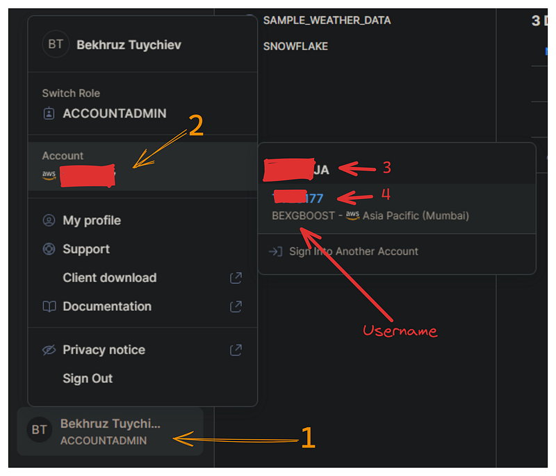
Now, we must establish a connection between Snowpark’s API and Snowflake’s cloud to query our database. This connection requires the following Snowflake credentials: account name, username, and password.

In the image below, I’ll show how you can retrieve your username and account name from the Snowflake dashboard:

Create a separate file named config.py that contains a single dictionary named credentials with the following format:

credentials = (
   {
       "account": "3-4",  # Combine 3 and 4 with a hyphen
       "username": "bexgboost",  # Your username in lowercase
       "password": "your_password",  # Your Snowflake password
   },
)

For security reasons, we store credentials in a separate file. Adding this file to .gitignore ensures that your Snowflake credentials won't be accidentally leaked.

Now, we import the credentials dictionary and the Session class of Snowpark:

from config import credentials
from snowflake.snowpark import Session

To establish a connection, we'll use the Session.builder.configs.create() method:

connection_parameters = {
   "account": credentials["account"],
   "user": credentials["username"],
   "password": credentials["password"],
}

new_session = Session.builder.configs(connection_parameters).create()
new_session.get_current_user()

'"bexgboost"'

If your username is printed, your first session is successfully created!

Loading the ingested data into a session

The new_session object has access to everything your account owns in Snowflake (and what you have permission to access).

The first step we'll do before importing data is to tell the session that we are using the test_db database we have created in the previous section:

new_session.sql("USE DATABASE test_db;").collect()

[Row(status='Statement executed successfully.')]

We do this using the .sql method, which allows us to run any Snowflake SQL-compatible query.

Now, we can load the diamonds table of test_db using the table method of the session object:

diamonds_df = new_session.table("diamonds")
diamonds_df.show(5)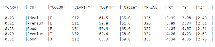

The .show() method is the equivalent of Pandas’ DataFrame.describe(), and it shows us that we have successfully connected to the table.

That's right - we only connected to the diamonds table. The diamonds_df object doesn't hold any data as evidenced by its size:

import sys
sys.getsizeof(diamonds_df)

48

It is only 48 bytes when it should have been over 3 MBs. Let’s spend a bit more time to understand why this is happening.

Understanding Snowpark DataFrames

So far, we’ve covered the following steps:

1. Created a virtual environment with relevant libraries.
2. Ingested sample data into Snowflake.
3. Created a Snowpark session to connect to Snowflake.

Let’s now discuss Snowpark DataFrames!

Snowpark DataFrames are lazy

Pandas DataFrames use your RAM, which means they live on your machine. In comparison, Snowpark DataFrames live within Snowflake’s cloud platform, even though you can see their representation in your coding environment. The data stays on the cloud and doesn’t need to be downloaded to your local machine to do operations on it.

Another important aspect of Snowpark DataFrames is that they work lazily. This means they don’t execute any operations on the data until you specifically tell them to.

Instead, they build a logical representation of the desired operations that are then translated into optimized SQL queries for Snowflake to execute.

By comparison, Pandas executes operations immediately—in other words, it performs eager execution.

Performance-wise, lazy evaluation is always significantly faster than eager execution. Since lazy DataFrames use Snowflake’s powerful elastic computing resources, they can push operations down to the database level and run much quicker.

To better understand the difference between lazy evaluation and eager execution, imagine that our data in Snowflake is a giant library. We have the following two scenarios:

• Eager execution (Pandas DataFrames): We gather all the books we need to our desk (local machine) and then analyze them individually.
• Lazy evaluation (Snowpark DataFrames): We tell the librarian (Snowpark) which books we need and what analysis we want to perform, and then the librarian retrieves and analyzes the relevant information efficiently.

When to use Snowpark DataFrames

Since Snowpark can convert to Pandas DataFrames, when should we use one over the other?

pandas_diamonds = diamonds_df.to_pandas()
pandas_diamonds.head()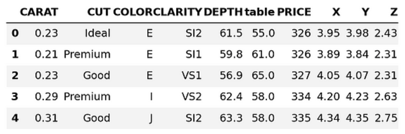

The answer largely depends on the size of the dataset.

If your dataset is small (like the Diamonds dataset), you can download it locally and feed it into Pandas without problems (which is what the DataFrame.to_pandas() method does).

But with today's datasets, things can quickly get out of hand and we may have to wait hours for our database to download. And remember, it is a two-way ticket—any new data we want to preserve must also be sent back. And that’s what makes learning the Snowpark DataFrame API so valuable.

Alternatively, the Session.sql() method allows us to execute any SQL expression compatible with Snowflake (see the example below). However, I strongly recommend mastering the Snowpark DataFrame API because it has many built-in functions for over 100 SQL functions and expressions.

result = new_session.sql(
   """
   SELECT PRICE, CUT FROM DIAMONDS LIMIT 10
"""
)

type(result)

snowflake.snowpark.dataframe.DataFrame

result.show()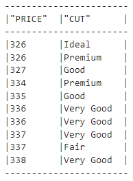

Snowpark DataFrame transformation functions

Much of your time in Snowpark will be spent using its transformation functions. They are available under the following sub-module:

# The convention is to import it as F
import snowflake.snowpark.functions as F

All functions under F (which you can list by calling dir(F)) specify how a DataFrame should be transformed. Let's look at an example:

F.upper(F.col("CUT"))

Here, the col function creates a reference to the given column and returns a Column object. Then, .upper() converts the values of the CUT column to uppercase:

diamonds_df.show(5)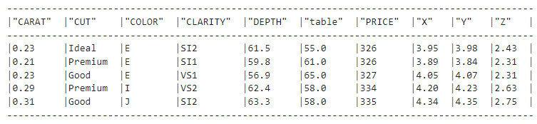

But if we look at the diamonds dataset, we see that the values in the CUT column still have lowercase letters. Why is that? Well, the F.upper(F.col("CUT")) expression is equivalent to the following SQL query:

SELECT UPPER(CUT);

What is missing here?

Of course, the FROM clause which specifies the table name the transformation should be applied to!

So, we must combine the F.upper(F.col("CUT")) expression with the diamonds_df object. There are three main ways to do this:

• For expressions that transform or select columns, pass inside .select()
• For expressions that select rows, pass inside .filter()
• For expressions that create columns, pass inside .with_column()

Since our expression transforms a column, we'll pass it to .select():

our_expression = F.upper(F.col("CUT"))
diamonds_df.select(our_expression).show()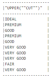

We changed the values successfully!

Let’s now write an expression that filters rows:

diamonds_df.filter(F.col("PRICE") > 10000).count()

5222

We find that there are over 5000 diamonds in our dataset that cost over $10,000. Let’s try creating a column as well:

(
diamonds_df.with_column("PRICE_SQUARED", F.col("PRICE") ** 2)
.select("PRICE", "PRICE_SQUARED")
.show(5)
)

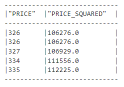
Above, we show that chaining methods are also allowed—we have a new column named “PRICE_SQUARED.” We see that Snowpark DataFrame’s functions are similar to Pandas’.

In summary, if you’re looking for a Snowpark alternative to a Pandas function, it’s either under F or part of the Snowpark DataFrames’ methods. You can check by calling dir(F) or dir(diamonds_df) or reading the Snowpark Python reference.

Performing EDA on Snowpark DataFrames

A significant part of performing exploratory data analysis (EDA) is creating visuals. Lucky for us, we don’t need Snowpark for this because we can keep using the modern data stack.

Here’s the idea : Since EDA is all about discovering general trends and insights, we can often use a sample instead of the entire dataset. Once we download a representative sample, we can convert it to Pandas DataFrame and use the good old Matplotlib or Seaborn.

Let’s start with the conversion:

sample = diamonds_df.sample(0.25).to_pandas()
sample.head()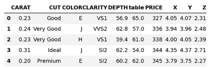

Above, we are downloading 25% of the dataset as a Pandas DataFrame. Let’s convert the column names to lowercase:

sample.columns = [col.lower() for col in sample.columns]
sample.columns

Index(['carat', 'cut', 'color', 'clarity', 'depth', 'table', 'price', 'x', 'y', 'z'], dtype='object')

Now, you can do EDA as you would on any dataset. Below, we explore a few possible ideas and start by generating a scatter plot to visualize the relationship between price and carat:

#Remember we imported seaborn as sns
sns.scatterplot(data=sample, x="price", y="carat", s=1)
plt.title("Diamond prices vs. carat")
plt.show()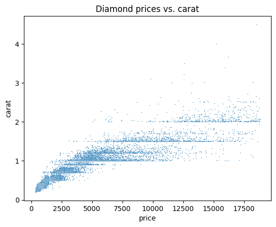

Let’s now plot a correlation matrix to see the correlation between every pair of numeric features:

corr_matrix = sample.corr(numeric_only=True)
sns.heatmap(corr_matrix, center=0, square=True, annot=True
plt.title("The correlation matrix of Diamond numeric features")
plt.show()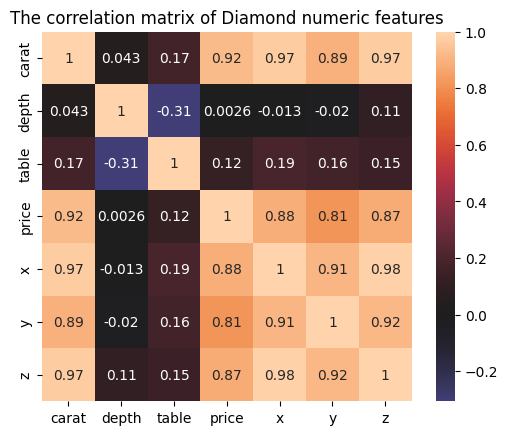

We could also create a bar plot of diamond cut categories:

cut_counts = sample.groupby("cut")["cut"].count()
cut_counts.plot(kind="bar")
plt.title("Category counts of diamond cuts")
plt.xlabel("Diamond cut")
plt.show()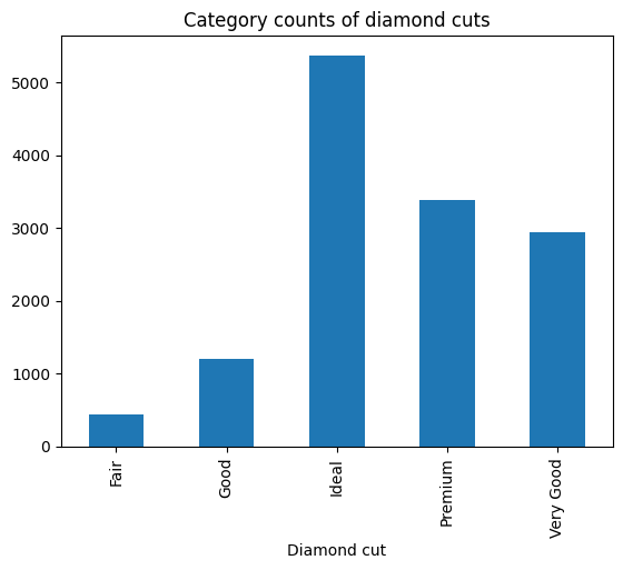

To confirm that these plots will be roughly the same on the entire dataset, we'll run the SQL version of the bar plot above.

First, we'll write an SQL expression to group the diamonds dataset by CUT:

result = new_session.sql(
   """
   SELECT cut, COUNT(*) AS count
     FROM diamonds
    GROUP BY cut;
"""
)

Let’s now convert and download the result as a Pandas DataFrame:

result_pd = result.to_pandas()
result_pd

This time, we'll use the plt.bar() function to create the graph:

plt.bar(x=result_pd["CUT"], height=result_pd["COUNT"])
plt.show()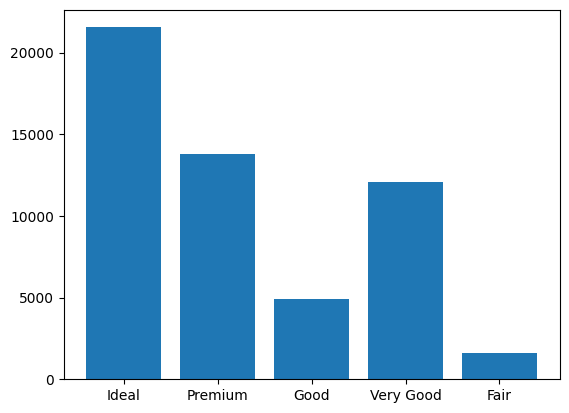

The order of bars is different but looking at them side-by-side reveals that they convey the same information.

Training a Machine Learning Model in Snowpark

We’re now ready to learn how to train machine learning models in Snowpark!

We'll start by cleaning the dataset.

Cleaning data in Snowpark

First, let’s make sure all the columns have the correct data type:

list(diamonds_df.schema)

[StructField('CARAT', DecimalType(38, 2), nullable=True),
StructField('CUT', StringType(16777216), nullable=True),
StructField('COLOR', StringType(16777216), nullable=True),
StructField('CLARITY', StringType(16777216), nullable=True),
StructField('DEPTH', DecimalType(38, 1), nullable=True),
StructField('"table"', DecimalType(38, 1), nullable=True),
StructField('PRICE', LongType(), nullable=True),
StructField('X', DecimalType(38, 2), nullable=True),
StructField('Y', DecimalType(38, 2), nullable=True),
StructField('Z', DecimalType(38, 2), nullable=True)]

The table column has a weird name, so we'll convert it to uppercase TABLE_ (with a trailing underscore so that it doesn't clash with a built-in SQL keyword):

diamonds_df = diamonds_df.with_column_renamed('"table"', "TABLE_")
diamonds_df.columns

['CARAT', 'CUT', 'COLOR', 'CLARITY', 'DEPTH', 'TABLE_', 'PRICE', 'X', 'Y', 'Z']

We’ll need to change the data type of numeric features from DecimalType to DoubleType because decimals aren't supported in Snowpark yet.

from snowflake.snowpark.types import DoubleType

numeric_features = ["CARAT", "X", "Y", "Z", "DEPTH", "TABLE_"]
for col in numeric_features:
   diamonds_df = diamonds_df.with_column(col, diamonds_df[col].cast(DoubleType()))

list(diamonds_df.select(*numeric_features))

[Column("CARAT"),
Column("X"),
Column("Y"),
Column("Z"),
Column("DEPTH"),
Column("TABLE_")]

In the snippet above, we use the .with_column() method again. Another new method is .cast(), which is part of Snowpark DataFrames' methods.

Snowpark also requires that all text features be uppercase and not have spaces between words before encoding them. Currently, the values of the CUT feature violate this requirement, so we'll fix it with function transformations:

import snowflake.snowpark.functions as F

def remove_space_and_upper(df):
   df = df.with_column("CUT", F.upper(F.replace(F.col("CUT"), " ", "_")))

   return df

diamonds_df = remove_space_and_upper(diamonds_df)

Our data is now free of cleaning issues. We can save it back as a new table to Snowflake:

diamonds_df.write.mode("overwrite").save_as_table("diamonds_cleaned")

Be sure to add the overwrite mode as you might have to go back and change some cleaning operations and save again.

Preparing data for modeling in Snowpark

In this section, we'll tackle any remaining pre-processing issues that might prevent models from training. Let’s load the cleaned table from the previous section:

clean_df = new_session.table("diamonds_cleaned")
clean_df.show()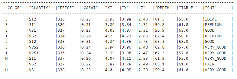

Very good!

Next, we'll import the preprocessing and pipeline sub-modules from the snowflake.ml namespace.

import snowflake.ml.modeling.preprocessing as snowml
from snowflake.ml.modeling.pipeline import Pipeline

While the DataFrame API of Snowpark is available under snowflake.snowpark, Snowpark ML modules are present in snowflake.ml. This might be confusing initially, so take your time to get used to it.

In the code below, we:

• List the categorical feature names that need to be encoded.
• Define names for output features because Snowpark adds the encoded features as new columns instead of replacing the old ones.
• Define the correct order of ordinal categories; in the diamonds dataset, all categories have inherent ordering, making them more expensive as you go from left to right.

# List all the features for processing
cat_cols = ["CUT", "COLOR", "CLARITY"]
cat_cols_encoded = ["CUT_OE", "COLOR_OE", "CLARITY_OE"]

# We already have numeric_features

# List the correct ordering of categorical features
categories = {
   "CUT": np.array(["IDEAL", "PREMIUM", "VERY_GOOD", "GOOD", "FAIR"]),
   "CLARITY": np.array(
       ["IF", "VVS1", "VVS2", "VS1", "VS2", "SI1", "SI2", "I1", "I2", "I3"]
   ),
   "COLOR": np.array(["D", "E", "F", "G", "H", "I", "J"]),
}

We're now ready to build a pipeline that is similar to a Scikit-learn pipeline:

# Build the pipeline
preprocessing_pipeline = Pipeline(
   steps=[
       (
           "OE",
           snowml.OrdinalEncoder(
               input_cols=cat_cols, output_cols=cat_cols_encoded, categories=categories
           ),
       ),
       (
           "SS",
           snowml.StandardScaler(
               input_cols=numeric_features, output_cols=numeric_features
           ),
       ),
   ]
)

The Pipeline class accepts a list of steps, each a pre-processing class. Here, we're using OrdinalEncoder to encode categoricals as 0, 1, 3, etc. and StandardScaler to normalize the numeric features.

In the end, we'll save the pipeline locally with joblib and test it on the entire dataset:

import joblib
PIPELINE_FILE = "pipeline.joblib"

# Pickle locally first
joblib.dump(preprocessing_pipeline, PIPELINE_FILE)

transformed_diamonds_df = preprocessing_pipeline.fit(clean_df).transform(clean_df)

# transformed_diamonds_df.show() - commented because of long output

The snippet runs without errors, so our pipeline is working, signaling we can finally train a model.

Training an XGBoost model in Snowpark

To train a model, we'll list the feature names and target names again:

# Define the columns again
cat_cols_encoded = ["CUT_OE", "COLOR_OE", "CLARITY_OE"]
numeric_features = ["CARAT", "X", "Y", "Z", "DEPTH", "TABLE_"]

label_cols = ["PRICE"]  # Must be a list
output_cols = ["PRICE_PREDICTED"]  # Required in snowpark

We'll now split the data using DataFrame.random_split() and give weights to represent the fraction of training and testing sets:

# Split the data
train_df, test_df = diamonds_df.random_split(weights=[0.8, 0.2], seed=42)

Then, we'll load the pipeline and fit-transform both train and test sets.

# Load the pre-processing pipeline locally
pipeline = joblib.load("pipeline.joblib")

# Apply it to both dataframes
train_df_transformed = pipeline.fit(train_df).transform(train_df)
test_df_transformed = pipeline.transform(test_df)

Above, make sure you call only .transform() on the test set to avoid data leakage.

Next, we initialize an XGBoost regressor model from ml.modeling.xgboost sub-module:

# Snowpark has models from scikit-learn and lightgbm too
from snowflake.ml.modeling.xgboost import XGBRegressor

# Initialize
regressor = XGBRegressor(
   input_cols=cat_cols_encoded + numeric_features,
   label_cols=label_cols,
   output_cols=output_cols,
)

The XGBRegressor class requires all input names, all target names, and output column names. Once we input them, we call .fit() to start the training process:

# Train
regressor.fit(train_df_transformed)

The training might run slowly if you have a free Snowflake account that has limited computing resources and no GPU.

Once the training finishes, we can generate predictions:

# Predict

train_preds = regressor.predict(train_df_transformed)
test_preds = regressor.predict(test_df_transformed)

Let’s take a look at the predictions:

train_preds.select("PRICE", "PRICE_PREDICTED").show(5)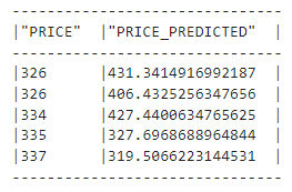

We now have to measure how well our initial model did. Snowpark includes dozens of metrics from Scikit-learn under its ml.modeling.metrics submodule which we we import as M:

import snowflake.ml.modeling.metrics as M

Then, we run mean_squared_error twice to measure root mean squared error (RMSE) on both training and test sets (below, squared=False returns RMSE instead of MSE):

rmse_train = M.mean_squared_error(
   df=train_preds,
   y_true_col_names=label_cols,
   y_pred_col_names=output_cols,
   squared=False,
)

rmse_test = M.mean_squared_error(
   df=test_preds,
   y_true_col_names=label_cols,
   y_pred_col_names=output_cols,
   squared=False,
)

print(f"Train RMSE score for XGBRegressor: {rmse_train:.4f}")
print(f"Test RMSE score for XGBRegressor: {rmse_test:.4f}")

Train RMSE score for XGBRegressor: 371.9664
Test RMSE score for XGBRegressor: 542.1566

Our model is off $542 on average and it might also be overfitting a bit because the difference between training and test RMSEs is large.

Let’s tune the hyperparameters of the model to tackle these issues.

Hyperparameter tuning in Snowpark

Currently, Snowpark offers two hyperparameter tuning classes:

• GridSearchCV: exhaustive search of all hyperparameter combinations with cross-validation.
• RandomizedSearchCV: randomized search of a given hyperparameter distributions with cross-validation.

XGBoost has about a dozen hyperparameters that can improve its performance (you can learn more in this tutorial on using XGBoost in Python). This pushes us to do a randomized search. Personally, I’d prefer to use Optuna which uses Bayesian search but we don’t have that luxury in Snowpark yet.

Let’s define the search now:

from snowflake.ml.modeling.model_selection import RandomizedSearchCV

rscv = RandomizedSearchCV(
   estimator=XGBRegressor(),
   param_distributions={
       "n_estimators": [2000],
       "max_depth": list(range(3, 13)),
       "learning_rate": np.linspace(0.1, 0.5, num=10),
   },
   n_jobs=-1,
   scoring="neg_mean_squared_error",
   input_cols=numeric_features + cat_cols_encoded,
   label_cols=label_cols,
   output_cols=output_cols,
   n_iter=10,
)

rscv.fit(train_df_transformed)

We're fixing the number of estimators to 2000 and only tuning max_depth and learning_rate parameters. The rscv has a default parameter of n_iter=10, which means the search will be performed 10 times, each time choosing a random combination of parameters. For more accurate results, it is best to choose a larger number for this parameter.

Now, let’s measure the performance of the best model found. The code is the same as before but instead of regressor, we'll use the rscv object:

# Predict
train_preds = rscv.predict(train_df_transformed)
test_preds = rscv.predict(test_df_transformed)
rmse_train = M.mean_squared_error(
   df=train_preds,
   y_true_col_names=label_cols,
   y_pred_col_names=output_cols,
   squared=False,
)

optimal_rmse_test = M.mean_squared_error(
   df=test_preds,
   y_true_col_names=label_cols,
   y_pred_col_names=output_cols,
   squared=False,
)

print(f"Train RMSE score for optimal model: {rmse_train:.4f}")
print(f"Test RMSE score for optimal model: {rmse_test:.4f}")

Train RMSE score for optimal model: 224.2405
Test RMSE score for optimal model: 572.0517

The training RMSE went down but the test RMSE is even larger. This dictates that we're still overfitting and we need to expand our search and include other parameters to prune the decision trees that XGBoost uses under the hood.

I will leave that part to you.

Saving the best model in Snowpark

If we close the session now, we'll lose our tuned model. To save it, we'll use Snowpark’s native model registry, which is a virtual storage that you can use to save any model and its metadata.

The registry is available as the Registry class, and it requires the current session's database and schema names. It also requires us to give the project a name so that we don’t run into conflicts with models from other projects:

# Set up for Registry
from snowflake.ml.registry import Registry

# Get the current db and schema name
db_name = new_session.get_current_database()
schema_name = new_session.get_current_schema()

# Define global model name for the project
model_name = "diamond_prices_regression"

# Initialize a registry to log models
registry = Registry(session=new_session, database_name=db_name, schema_name=schema_name)

We'll use the Registry.log_model() method to save our models:

# Get sample data to pass into registry for schema
sample = train_df.select(cat_cols_encoded + numeric_features).limit(50)

# Log the first model
v0 = registry.log_model(
   model_name=model_name,
   version_name="v0",
   model=regressor,
   sample_input_data=sample,
)

We can log a metric for the model with .set_metric() method (we can log as many metrics as we want). We'll also add a comment to describe the model:

# Add the models RMSE score
v0.set_metric(metric_name="RMSE", value=rmse_test)

# Add a description
v0.comment = "The first model to predict diamond prices"

We do the same for the best model found with random search. While logging the metric, don’t forget to change the value to optimal_rmse_test.

# Log the optimal model
v1 = registry.log_model(
   model_name=model_name,
   version_name="v1",
   model=regressor,
   sample_input_data=sample,
)

# Add the models RMSE score
v1.set_metric(metric_name="RMSE", value=optimal_rmse_test)

# Add a description
v1.comment = "Optimal model found with RandomizedSearchCV"

To confirm that the models are saved, you can call .show_models():

# Confirm the models are added
registry.show_models()

Learn more about how to manage the registry from this page of the developer docs on Snowpark.

Doing inference in Snowpark

Inference is usually done by choosing the best model from your registry. We can do that by filtering the result of .show_models() or by retrieving the model directly with its version tag as we do below:

# Doing inference with the optimal model
optimal_version = registry.get_model(model_name).version("v1")
results = optimal_version.run(test_df, function_name="predict")

results.columns

The get_model() method returns a generic model object, which is different from XGBRegressor. That's why you have to call .run() by specifying the function name to perform an inference.

Conclusion

In this tutorial, we covered an end-to-end framework to train machine learning models in Snowflake Snowpark. Well done!

We started off with a bare-bones uncleaned dataset and ended up with a tuned XGBoost regressor model. We’ve performed all actions on Snowflake Cloud, which means we didn’t have to use system resources at all.

We’ve learned how effective this type of in-database operations are when we have large datasets—and that Snowflake Snowpark is one of the best tools in the market to facilitate this process.

If you want to learn more about Snowpark or Snowflake, check the following resources:

• Using Snowflake Time Travel: A Comprehensive Guide
• Getting Started with Data Analysis in Snowflake using Python and SQL
• The Best Snowflake Certification For 2024
• Snowpark API Developer Guide — a must-read
• Snowpark ML Developer Guide

Thank you for reading!