Implementing Autoencoders in Keras: Tutorial

Generally, you can consider autoencoders as an unsupervised learning technique, since you don’t need explicit labels to train the model on. All you need to train an autoencoder is raw input data.

In this tutorial, you’ll learn about autoencoders in deep learning and you will implement a convolutional and denoising autoencoder in Python with Keras. You will work with the NotMNIST alphabet dataset as an example.

In a nutshell, you'll address the following topics in today's tutorial:

• You'll first learn more about autoencoders: what they are, how they compare to dimensionality reduction techniques, and the different types that you can find of this algorithm;
• Next, you'll focus on the convolutional autoencoder: you'll first see what this type of autoencoder does and how you can construct it. Afterwards, you'll implement one yourself! You'll learn how to load the data when it is in ubyte gzip format, then you'll explore the data, preprocess the data, fit the data in a model, visualize the training and validation loss plot and finally predict on the test set.
• Next, you'll will be introduced to denoising autoencoder and you'll see how you can implement one: you'll learn to add noise to the images. Next, you'll feed these images into your deep learning model and train it! Finally, you'll predict on the noisy test images.

Autoencoder

As you read in the introduction, an autoencoder is an unsupervised machine learning algorithm that takes an image as input and tries to reconstruct it using fewer number of bits from the bottleneck also known as latent space. The image is majorly compressed at the bottleneck. The compression in autoencoders is achieved by training the network for a period of time and as it learns it tries to best represent the input image at the bottleneck. The general image compression algorithms like JPEG and JPEG lossless compression techniques compress the images without the need for any kind of training and do fairly well in compressing the images.

Autoencoders are similar to dimensionality reduction techniques like Principal Component Analysis (PCA). They project the data from a higher dimension to a lower dimension using linear transformation and try to preserve the important features of the data while removing the non-essential parts.

However, the major difference between autoencoders and PCA lies in the transformation part: as you already read, PCA uses linear transformation whereas autoencoders use non-linear transformations.

Now that you have a bit of understanding about autoencoders, let's now break this term and try to get some intuition about it!

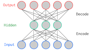
The above figure is a two-layer vanilla autoencoder with one hidden layer. In deep learning terminology, you will often notice that the input layer is never taken into account while counting the total number of layers in an architecture. The total layers in an architecture only comprises of the number of hidden layers and the ouput layer.

As shown in the image above, the input and output layers have the same number of neurons.

Let's take an example. You feed an image with just five pixel values into the autoencoder which is compressed by the encoder into three pixel values at the bottleneck (middle layer) or latent space. Using these three values, the decoder tries to reconstruct the five pixel values or rather the input image which you fed as an input to the network.

In reality, there are more number of hidden layers in between the input and the output.

Autoencoder can be broken in to three parts

• Encoder: this part of the network compresses or downsamples the input into a fewer number of bits. The space represented by these fewer number of bits is often called the latent-space or bottleneck. The bottleneck is also called the "maximum point of compression" since at this point the input is compressed the maximum. These compressed bits that represent the original input are together called an “encoding” of the input.
• Decoder: this part of the network tries to reconstruct the input using only the encoding of the input. When the decoder is able to reconstruct the input exactly as it was fed to the encoder, you can say that the encoder is able to produce the best encodings for the input with which the decoder is able to reconstruct well!

There are variety of autoencoders, such as the convolutional autoencoder, denoising autoencoder, variational autoencoder and sparse autoencoder. However, as you read in the introduction, you'll only focus on the convolutional and denoising ones in this tutorial.Convolutional Autoencoders in Python with Keras

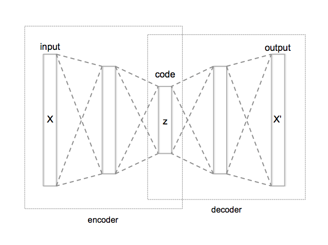
Since your input data consists of images, it is a good idea to use a convolutional autoencoder. It is not an autoencoder variant, but rather a traditional autoencoder stacked with convolution layers: you basically replace fully connected layers by convolutional layers. Convolution layers along with max-pooling layers, convert the input from wide (a 28 x 28 image) and thin (a single channel or gray scale) to small (7 x 7 image at the latent space) and thick (128 channels).

Do not worry if you did not understand the above idea properly! The second part of this tutorial, in which you'll focus on the implementation of the above, will hopefully clear all your doubts (if you have any!).

Tip: if you want to know more about convolutional neural networks, check out this tutorial.

This helps the network to extract visual features from the images and therefore obtain a more accurate latent space representation. The reconstruction process uses upsampling and convolutions which are known as a decoder. The downsampling is the process in which the image compresses into a low dimension also known as an encoder.

It is important to note that the encoder mainly compresses the input image, for example: if your input image is of dimension 176 x 176 x 1 (~30976), then the maximum compression point can have a dimension of 22 x 22 x 512 (~247808). So, in this case, you started with a gray scale image of dimension 176 x 176 and by passing it through a couple of convolutional layers and precisely three max-pooling layers, your image is finally downsampled to a dimension of 22 x 22 but the number of channels are increased from 1 to 512. As stated above, your input from wide (176 x 176) and thin (1) became small (22x22) and thick (512).

Loading the Data

The notMNIST dataset is an image recognition dataset of font glypyhs for the letters A through J. It is quite similar to the classic MNIST dataset, which contains images of handwritten digits 0 through 9: in this case, you'll find that the NotMNIST dataset comprises 28x28 grayscale images of 70,000 letters from A - J in total 10 categories, and 6,000 images per category.

Tip: if you want to learn how to implement an Multi-Layer Perceptron (MLP) for classification tasks with the MNIST dataset, check out this tutorial.

The NotMNIST dataset is not predefined in the Keras or the TensorFlow framework, so you'll have to download the data from this source. The data will be downloaded in ubyte.gzip format, but no worries about that just yet! You'll soon learn how to read bytestream formats and convert them into a NumPy array. So, let's get started!

The network will be trained on a Nvidia Tesla K40, so if you train on a GPU and use Jupyter Notebook, you will need to add three more lines of code where you specify CUDA device order and CUDA visible devices using a module called os.

In the code below, you basically set environment variables in the notebook using os.environ. It's good to do the following before initializing Keras to limit Keras backend TensorFlow to use first GPU. If the machine on which you train on has a GPU on 0, make sure to use 0 instead of 1. You can check that by running a simple command on your terminal: for example, nvidia-smi

import os
os.environ["CUDA_DEVICE_ORDER"]="PCI_BUS_ID"
os.environ["CUDA_VISIBLE_DEVICES"]="1" #model will be trained on GPU 1

Next, you import all the required modules like numpy, matplotlib and most importantly keras, since you'll be using that framework in today's tutorial!

import keras
from matplotlib import pyplot as plt
import numpy as np
import gzip
%matplotlib inline
from keras.layers import Input,Conv2D,MaxPooling2D,UpSampling2D
from keras.models import Model
from keras.optimizers import RMSprop

Using TensorFlow backend.

Here, you define a function that opens the gzip file, reads the file using bytestream.read(). You pass the image dimension and the total number of images to this function. Then, using np.frombuffer(), you convert the string stored in variable buf into a NumPy array of type float32.

Next, you reshape the array into a three-dimensional array or tensor where the first dimension is number of images, and the second and third dimension being the dimension of the image. Finally, you return the NumPy array data.

def extract_data(filename, num_images):
    with gzip.open(filename) as bytestream:
        bytestream.read(16)
        buf = bytestream.read(28 * 28 * num_images)
        data = np.frombuffer(buf, dtype=np.uint8).astype(np.float32)
        data = data.reshape(num_images, 28,28)
        return data

You will now call the function extract_data() by passing the training and testing files along with their corresponding number of images:

train_data = extract_data('train-images-idx3-ubyte.gz', 60000)
test_data = extract_data('t10k-images-idx3-ubyte.gz', 10000)

Similarly, you define a extract labels function that opens the gzip file, reads the file using bytestream.read(), to which you pass the label dimension (1) and the total number of images. Then, using np.frombuffer(), you convert the string stored in variable buf into a NumPy array of type int64.

This time, you do not need to reshape the array since the variable labels will return a column vector of dimension 60,000 x 1. Finally, you return the NumPy array labels.

def extract_labels(filename, num_images):
    with gzip.open(filename) as bytestream:
        bytestream.read(8)
        buf = bytestream.read(1 * num_images)
        labels = np.frombuffer(buf, dtype=np.uint8).astype(np.int64)
        return labels

You will now call the function extract label by passing the training and testing label files along with their corresponding number of images:

train_labels = extract_labels('train-labels-idx1-ubyte.gz',60000)
test_labels = extract_labels('t10k-labels-idx1-ubyte.gz',10000)

Once you have the training and testing data loaded, you are all set to analyze the data in order to get some intuition about the dataset that you are going to work with for today's tutorial!

Data Exploration

Let's now analyze how images in the dataset look like and also see the dimension of the images with the help of the NumPy array attribute .shape:

# Shapes of training set
print("Training set (images) shape: {shape}".format(shape=train_data.shape))

# Shapes of test set
print("Test set (images) shape: {shape}".format(shape=test_data.shape))

Training set (images) shape: (60000, 28, 28)
Test set (images) shape: (10000, 28, 28)

From the above output, you can see that the training data has a shape of 60000 x 28 x 28 since there are 60,000 training samples each of 28 x 28 dimensional matrix. Similarly, the test data has a shape of 10000 x 28 x 28 since there are 10,000 testing samples.

Note that in this task, you will not be using the training and testing labels. The task at hand will only be dealing with the training and testing images. However, for exploration purposes, which might give you a better intuition about the data, you'll make use the labels.

Let's create a dictionary that will have class names with their corresponding categorical class labels:

# Create dictionary of target classes
label_dict = {
 0: 'A',
 1: 'B',
 2: 'C',
 3: 'D',
 4: 'E',
 5: 'F',
 6: 'G',
 7: 'H',
 8: 'I',
 9: 'J',
}

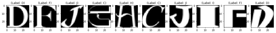
Now, let's take a look at couple of the images in your dataset:

plt.figure(figsize=[5,5])

# Display the first image in training data
plt.subplot(121)
curr_img = np.reshape(train_data[0], (28,28))
curr_lbl = train_labels[0]
plt.imshow(curr_img, cmap='gray')
plt.title("(Label: " + str(label_dict[curr_lbl]) + ")")

# Display the first image in testing data
plt.subplot(122)
curr_img = np.reshape(test_data[0], (28,28))
curr_lbl = test_labels[0]
plt.imshow(curr_img, cmap='gray')
plt.title("(Label: " + str(label_dict[curr_lbl]) + ")")

<matplotlib.text.Text at 0x7f3ec73db240>

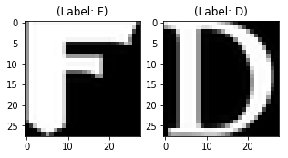
The output of above two plots are one of the sample images from both training and testing data, and these images are assigned a class label of 5 or F, on the one hand, and 3 or D, on the other hand. Similarly, other alphabets will have different labels, but similar alphabets will have same labels. This means that all the 6,000 class F images will have a class label of 5.

Data Preprocessing

The images of the dataset are indeed grayscale images with pixel values ranging from 0 to 255 with a dimension of 28 x 28 so before you feed the data into the model it is very important to preprocess it. You'll first convert each 28 x 28 image of train and test set into a matrix of size 28 x 28 x 1, which you can feed into the network:

train_data = train_data.reshape(-1, 28,28, 1)
test_data = test_data.reshape(-1, 28,28, 1)
train_data.shape, test_data.shape

((60000, 28, 28, 1), (10000, 28, 28, 1))

Next, you want to make sure to check the data type of the training and testing NumPy arrays, it should be in float32 format, if not you will need to convert it into this format, but since you already have converted it while reading the data you no longer need to do this again. You also have to rescale the pixel values in range 0 - 1 inclusive. So let's do that!

Don't forget to verify the training and testing data types:

train_data.dtype, test_data.dtype

(dtype('float32'), dtype('float32'))

Next, rescale the training and testing data with the maximum pixel value of the training and testing data:

np.max(train_data), np.max(test_data)

(255.0, 255.0)

train_data = train_data / np.max(train_data)
test_data = test_data / np.max(test_data)

Let's verify the maximum value of training and testing data which should be 1.0 after rescaling it!

np.max(train_data), np.max(test_data)

(1.0, 1.0)

After all of this, it's important to partition the data. In order for your model to generalize well, you split the training data into two parts: a training and a validation set. You will train your model on 80% of the data and validate it on 20% of the remaining training data.

This will also help you in reducing the chances of overfitting, as you will be validating your model on data it would not have seen in training phase.

You can use the train_test_split module of scikit-learn to divide the data properly:

from sklearn.model_selection import train_test_split
train_X,valid_X,train_ground,valid_ground = train_test_split(train_data,
                                                             train_data, 
                                                             test_size=0.2, 
                                                             random_state=13)

Note that for this task, you don't need training and testing labels. That's why you will pass the training images twice. Your training images will both act as the input as well as the ground truth similar to the labels you have in classification task.

Now you are all set to define the network and feed the data into the network. So without any further ado, let's jump to the next step!

The Convolutional Autoencoder

The images are of size 28 x 28 x 1 or a 784-dimensional vector. You convert the image matrix to an array, rescale it between 0 and 1, reshape it so that it's of size 28 x 28 x 1, and feed this as an input to the network.

Also, you will use a batch size of 128 using a higher batch size of 256 or 512 is also preferable it all depends on the system you train your model. It contributes heavily in determining the learning parameters and affects the prediction accuracy. You will train your network for 50 epochs.

batch_size = 128
epochs = 50
inChannel = 1
x, y = 28, 28
input_img = Input(shape = (x, y, inChannel))

As discussed before, the autoencoder is divided into two parts: there's an encoder and a decoder.

Encoder

• The first layer will have 32 filters of size 3 x 3, followed by a downsampling (max-pooling) layer,
• The second layer will have 64 filters of size 3 x 3, followed by another downsampling layer,
• The final layer of encoder will have 128 filters of size 3 x 3.

Decoder

• The first layer will have 128 filters of size 3 x 3 followed by a upsampling layer,/li>
• The second layer will have 64 filters of size 3 x 3 followed by another upsampling layer,
• The final layer of encoder will have 1 filter of size 3 x 3.

The max-pooling layer will downsample the input by two times each time you use it, while the upsampling layer will upsample the input by two times each time it is used.

Note: The number of filters, the filter size, the number of layers, number of epochs you train your model, are all hyperparameters and should be decided based on your own intuition, you are free to try new experiments by tweaking with these hyperparameters and measure the performance of your model. And that is how you will slowly learn the art of deep learning!

def autoencoder(input_img):
    #encoder
    #input = 28 x 28 x 1 (wide and thin)
    conv1 = Conv2D(32, (3, 3), activation='relu', padding='same')(input_img) #28 x 28 x 32
    pool1 = MaxPooling2D(pool_size=(2, 2))(conv1) #14 x 14 x 32
    conv2 = Conv2D(64, (3, 3), activation='relu', padding='same')(pool1) #14 x 14 x 64
    pool2 = MaxPooling2D(pool_size=(2, 2))(conv2) #7 x 7 x 64
    conv3 = Conv2D(128, (3, 3), activation='relu', padding='same')(pool2) #7 x 7 x 128 (small and thick)

    #decoder
    conv4 = Conv2D(128, (3, 3), activation='relu', padding='same')(conv3) #7 x 7 x 128
    up1 = UpSampling2D((2,2))(conv4) # 14 x 14 x 128
    conv5 = Conv2D(64, (3, 3), activation='relu', padding='same')(up1) # 14 x 14 x 64
    up2 = UpSampling2D((2,2))(conv5) # 28 x 28 x 64
    decoded = Conv2D(1, (3, 3), activation='sigmoid', padding='same')(up2) # 28 x 28 x 1
    return decoded

After the model is created, you have to compile it using the optimizer to be RMSProp.

Tip: watch this tutorial by Andrew Ng on RMSProp if you want to get to know more about RMSProp.

Note that you also have to specify the loss type via the argument loss. In this case, that's the mean squared error, since the loss after every batch will be computed between the batch of predicted output and the ground truth using mean squared error pixel by pixel:

autoencoder = Model(input_img, autoencoder(input_img))
autoencoder.compile(loss='mean_squared_error', optimizer = RMSprop())

Let's visualize the layers that you created in the above step by using the summary function, this will show number of parameters (weights and biases) in each layer and also the total parameters in your model.

autoencoder.summary()

_________________________________________________________________
Layer (type)                 Output Shape              Param #   
=================================================================
input_6 (InputLayer)         (None, 28, 28, 1)         0         
_________________________________________________________________
conv2d_25 (Conv2D)           (None, 28, 28, 32)        320       
_________________________________________________________________
max_pooling2d_9 (MaxPooling2 (None, 14, 14, 32)        0         
_________________________________________________________________
conv2d_26 (Conv2D)           (None, 14, 14, 64)        18496     
_________________________________________________________________
max_pooling2d_10 (MaxPooling (None, 7, 7, 64)          0         
_________________________________________________________________
conv2d_27 (Conv2D)           (None, 7, 7, 128)         73856     
_________________________________________________________________
conv2d_28 (Conv2D)           (None, 7, 7, 128)         147584    
_________________________________________________________________
up_sampling2d_9 (UpSampling2 (None, 14, 14, 128)       0         
_________________________________________________________________
conv2d_29 (Conv2D)           (None, 14, 14, 64)        73792     
_________________________________________________________________
up_sampling2d_10 (UpSampling (None, 28, 28, 64)        0         
_________________________________________________________________
conv2d_30 (Conv2D)           (None, 28, 28, 1)         577       
=================================================================
Total params: 314,625
Trainable params: 314,625
Non-trainable params: 0
_________________________________________________________________

It's finally time to train the model with Keras' fit() function! The model trains for 50 epochs. The fit() function will return a history object; By storying the result of this function in fashion_train, you can use it later to plot the loss function plot between training and validation which will help you to analyze your model's performance visually.

Train the model

autoencoder_train = autoencoder.fit(train_X, train_ground, batch_size=batch_size,epochs=epochs,verbose=1,validation_data=(valid_X, valid_ground))

Train on 48000 samples, validate on 12000 samples
Epoch 1/50
48000/48000 [==============================] - 16s - loss: 0.0368 - val_loss: 0.0132
Epoch 2/50
48000/48000 [==============================] - 15s - loss: 0.0101 - val_loss: 0.0085
Epoch 3/50
48000/48000 [==============================] - 15s - loss: 0.0071 - val_loss: 0.0081
Epoch 4/50
48000/48000 [==============================] - 15s - loss: 0.0057 - val_loss: 0.0056
Epoch 5/50
48000/48000 [==============================] - 15s - loss: 0.0048 - val_loss: 0.0051
Epoch 6/50
48000/48000 [==============================] - 15s - loss: 0.0043 - val_loss: 0.0039
Epoch 7/50
48000/48000 [==============================] - 15s - loss: 0.0038 - val_loss: 0.0039
Epoch 8/50
48000/48000 [==============================] - 15s - loss: 0.0035 - val_loss: 0.0039
Epoch 9/50
48000/48000 [==============================] - 15s - loss: 0.0032 - val_loss: 0.0030
Epoch 10/50
48000/48000 [==============================] - 15s - loss: 0.0030 - val_loss: 0.0029
Epoch 11/50
48000/48000 [==============================] - 15s - loss: 0.0029 - val_loss: 0.0026
Epoch 12/50
48000/48000 [==============================] - 15s - loss: 0.0027 - val_loss: 0.0025
Epoch 13/50
48000/48000 [==============================] - 15s - loss: 0.0026 - val_loss: 0.0028
Epoch 14/50
48000/48000 [==============================] - 15s - loss: 0.0025 - val_loss: 0.0022
Epoch 15/50
48000/48000 [==============================] - 15s - loss: 0.0024 - val_loss: 0.0024
Epoch 16/50
48000/48000 [==============================] - 16s - loss: 0.0023 - val_loss: 0.0027
Epoch 17/50
48000/48000 [==============================] - 15s - loss: 0.0023 - val_loss: 0.0022
Epoch 18/50
48000/48000 [==============================] - 16s - loss: 0.0022 - val_loss: 0.0025
Epoch 19/50
48000/48000 [==============================] - 16s - loss: 0.0022 - val_loss: 0.0022
Epoch 20/50
48000/48000 [==============================] - 15s - loss: 0.0021 - val_loss: 0.0022
Epoch 21/50
48000/48000 [==============================] - 16s - loss: 0.0021 - val_loss: 0.0020
Epoch 22/50
48000/48000 [==============================] - 16s - loss: 0.0020 - val_loss: 0.0019
Epoch 23/50
48000/48000 [==============================] - 16s - loss: 0.0020 - val_loss: 0.0021
Epoch 24/50
48000/48000 [==============================] - 16s - loss: 0.0020 - val_loss: 0.0018
Epoch 25/50
48000/48000 [==============================] - 16s - loss: 0.0019 - val_loss: 0.0020
Epoch 26/50
48000/48000 [==============================] - 16s - loss: 0.0019 - val_loss: 0.0020
Epoch 27/50
48000/48000 [==============================] - 16s - loss: 0.0019 - val_loss: 0.0017
Epoch 28/50
48000/48000 [==============================] - 16s - loss: 0.0018 - val_loss: 0.0018
Epoch 29/50
48000/48000 [==============================] - 16s - loss: 0.0018 - val_loss: 0.0019
Epoch 30/50
48000/48000 [==============================] - 16s - loss: 0.0018 - val_loss: 0.0017
Epoch 31/50
48000/48000 [==============================] - 16s - loss: 0.0018 - val_loss: 0.0019
Epoch 32/50
48000/48000 [==============================] - 16s - loss: 0.0017 - val_loss: 0.0018
Epoch 33/50
48000/48000 [==============================] - 16s - loss: 0.0017 - val_loss: 0.0017
Epoch 34/50
48000/48000 [==============================] - 15s - loss: 0.0017 - val_loss: 0.0018
Epoch 35/50
48000/48000 [==============================] - 15s - loss: 0.0017 - val_loss: 0.0019
Epoch 36/50
48000/48000 [==============================] - 15s - loss: 0.0017 - val_loss: 0.0016
Epoch 37/50
48000/48000 [==============================] - 15s - loss: 0.0017 - val_loss: 0.0017
Epoch 38/50
48000/48000 [==============================] - 15s - loss: 0.0016 - val_loss: 0.0019
Epoch 39/50
48000/48000 [==============================] - 15s - loss: 0.0016 - val_loss: 0.0015
Epoch 40/50
48000/48000 [==============================] - 15s - loss: 0.0016 - val_loss: 0.0017
Epoch 41/50
48000/48000 [==============================] - 15s - loss: 0.0016 - val_loss: 0.0017
Epoch 42/50
48000/48000 [==============================] - 15s - loss: 0.0016 - val_loss: 0.0014
Epoch 43/50
48000/48000 [==============================] - 15s - loss: 0.0016 - val_loss: 0.0018
Epoch 44/50
48000/48000 [==============================] - 15s - loss: 0.0016 - val_loss: 0.0015
Epoch 45/50
48000/48000 [==============================] - 15s - loss: 0.0016 - val_loss: 0.0014
Epoch 46/50
48000/48000 [==============================] - 16s - loss: 0.0015 - val_loss: 0.0016
Epoch 47/50
48000/48000 [==============================] - 16s - loss: 0.0015 - val_loss: 0.0017
Epoch 48/50
48000/48000 [==============================] - 16s - loss: 0.0015 - val_loss: 0.0015
Epoch 49/50
48000/48000 [==============================] - 16s - loss: 0.0015 - val_loss: 0.0016
Epoch 50/50
48000/48000 [==============================] - 16s - loss: 0.0015 - val_loss: 0.0020

Finally! You trained the model on Not-MNIST for 50 epochs, Now, let's plot the loss plot between training and validation data to visualise the model performance.

Training vs Validation Loss Plot

loss = autoencoder_train.history['loss']
val_loss = autoencoder_train.history['val_loss']
epochs = range(epochs)
plt.figure()
plt.plot(epochs, loss, 'bo', label='Training loss')
plt.plot(epochs, val_loss, 'b', label='Validation loss')
plt.title('Training and validation loss')
plt.legend()
plt.show()

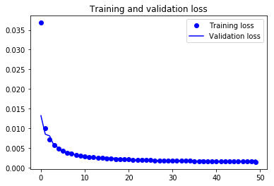
Finally, you can see that the validation loss and the training loss both are in sync. It shows that your model is not overfitting: the validation loss is decreasing and not increasing, and there rarely any gap between training and validation loss.

Therefore, you can say that your model's generalization capability is good.

Finally, it's time to reconstruct the test images using the predict() function of Keras and see how well your model is able reconstruct on the test data.

Predicting on Test Data

You will be predicting the trained model on the complete 10,000 test images and plot few of the reconstructed images to visualize how well your model is able to reconstruct the test images.

pred = autoencoder.predict(test_data)

pred.shape

(10000, 28, 28, 1)

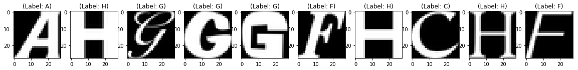
plt.figure(figsize=(20, 4))
print("Test Images")
for i in range(10):
    plt.subplot(2, 10, i+1)
    plt.imshow(test_data[i, ..., 0], cmap='gray')
    curr_lbl = test_labels[i]
    plt.title("(Label: " + str(label_dict[curr_lbl]) + ")")
plt.show()    
plt.figure(figsize=(20, 4))
print("Reconstruction of Test Images")
for i in range(10):
    plt.subplot(2, 10, i+1)
    plt.imshow(pred[i, ..., 0], cmap='gray')  
plt.show()

Test Images

Reconstruction of Test Images

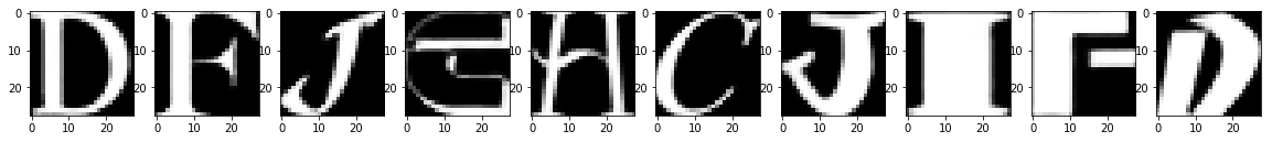
From the above figures, you can observe that your model did a fantastic job in reconstructing the test images that you predicted using the model. At least visually speaking, the test and the reconstructed images look almost exactly similar.

Denoising Autoencoder

A denoising autoencoder tries to learn a representation (latent-space or bottleneck) that is robust to noise. You add noise to an image and then feed the noisy image as an input to the enooder part of your network. The encoder part of the autoencoder transforms the image into a different space that tries to preserve the alphabets but removes the noise.

But how does it exactly remove the noise?

During training, you define a loss function, similar to the root mean squared error that you had defined earlier in convolutional autoencoder. At every iteration of the training, the network will compute a loss between the noisy image outputted by the decoder and the ground truth (denoisy image) and will also try to minimize that loss or difference between the reconstructed image and the original noise-free image. In other words, the network will learn a 7 x 7 x 128 space that will be noise free encodings of the data that you will train your network on!

Implementation of Denoising Autoencoder

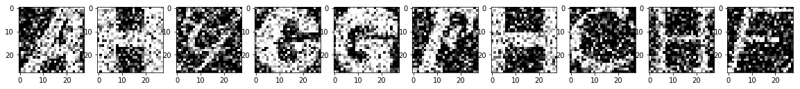
Now, to see how this works in Python, you will be using the same NotMNIST dataset as you did in the first part of this tutorial. That means you need not do any data preprocessing since it has already been done before! However, one important preprocessing step in this part of the tutorial will be adding noise to the training, validation and testing images. So, let's quickly do that first!

Adding Noise to Images

Let's first define a noise factor which is a hyperparameter. The noise factor is multiplied with a random matrix that has a mean of 0.0 and standard deviation of 1.0. This matrix will draw samples from normal (Gaussian) distribution. The shape of the random normal array will be similar to the shape of the data you will be adding the noise.

For simplicity, let's understand it with an example: The variable train_X has a shape of 48000 x 28 x 28 x 1. Hence, the random normal array will also have a shape similar to train_X only then you will be able to add two arrays since then they will have same dimensions.

noise_factor = 0.5
x_train_noisy = train_X + noise_factor * np.random.normal(loc=0.0, scale=1.0, size=train_X.shape)
x_valid_noisy = valid_X + noise_factor * np.random.normal(loc=0.0, scale=1.0, size=valid_X.shape)
x_test_noisy = test_data + noise_factor * np.random.normal(loc=0.0, scale=1.0, size=test_data.shape)
x_train_noisy = np.clip(x_train_noisy, 0., 1.)
x_valid_noisy = np.clip(x_valid_noisy, 0., 1.)
x_test_noisy = np.clip(x_test_noisy, 0., 1.)

np.clip() will threshold all the negative values to zero and all the values greater than one to one. Since, you want your pixel values to be between zero and one. And there are chances that after introducing noise into the data the pixel values range can change a bit, so to be on the safer side it's a good practice to clip the pixel values.

Visualizing the noisy images

plt.figure(figsize=[5,5])

# Display the first image in training data
plt.subplot(121)
curr_img = np.reshape(x_train_noisy[1], (28,28))
plt.imshow(curr_img, cmap='gray')

# Display the first image in testing data
plt.subplot(122)
curr_img = np.reshape(x_test_noisy[1], (28,28))
plt.imshow(curr_img, cmap='gray')

<matplotlib.image.AxesImage at 0x7f3ec6b20e48>

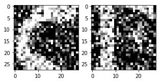
Now that you have the noisy data, you can feed it into the network and see how the noise is "magically" removed from the images!

Denoising Autoencoder Network

As discussed before the autoencoder is divided into two parts: the encoder and the decoder. The architecture that you're going to construct will look like the following:

Encoder

• The first layer will have 32-3 x 3 filters followed by a downsampling (max-pooling) layer,
• The second layer will have 64-3 x 3 filters followed by another downsampling layer,
• The final layer of encoder will have 128-3 x 3 filters.

Decoder

• The first layer will have 128-3 x 3 filters followed by a upsampling layer,
• The second layer will have 64-3 x 3 filters followed by another upsampling layer,
• The final layer of encoder will have 1-3 x 3 filters.

batch_size = 128
epochs = 20
inChannel = 1
x, y = 28, 28
input_img = Input(shape = (x, y, inChannel))

def autoencoder(input_img):
    #encoder
    conv1 = Conv2D(32, (3, 3), activation='relu', padding='same')(input_img)
    pool1 = MaxPooling2D(pool_size=(2, 2))(conv1)
    conv2 = Conv2D(64, (3, 3), activation='relu', padding='same')(pool1)
    pool2 = MaxPooling2D(pool_size=(2, 2))(conv2)
    conv3 = Conv2D(128, (3, 3), activation='relu', padding='same')(pool2)

    #decoder
    conv4 = Conv2D(128, (3, 3), activation='relu', padding='same')(conv3)
    up1 = UpSampling2D((2,2))(conv4)
    conv5 = Conv2D(64, (3, 3), activation='relu', padding='same')(up1)
    up2 = UpSampling2D((2,2))(conv5)
    decoded = Conv2D(1, (3, 3), activation='sigmoid', padding='same')(up2)
    return decoded

autoencoder = Model(input_img, autoencoder(input_img))
autoencoder.compile(loss='mean_squared_error', optimizer = RMSprop())

Training

If you remember while training the convolutional autoencoder, you had fed the training images twice since the input and the ground truth were both same. However, in denoising autoencoder, you feed the noisy images as an input while your ground truth remains the denoisy images on which you had applied the noise. Only then the network will be able to compute a loss between the noisy and the true denoisy images.

autoencoder_train = autoencoder.fit(x_train_noisy, train_X, batch_size=batch_size,epochs=epochs,verbose=1,validation_data=(x_valid_noisy, valid_X))

Train on 48000 samples, validate on 12000 samples
Epoch 1/20
48000/48000 [==============================] - 15s - loss: 0.0531 - val_loss: 0.0268
Epoch 2/20
48000/48000 [==============================] - 14s - loss: 0.0243 - val_loss: 0.0217
Epoch 3/20
48000/48000 [==============================] - 14s - loss: 0.0207 - val_loss: 0.0200
Epoch 4/20
48000/48000 [==============================] - 14s - loss: 0.0190 - val_loss: 0.0184
Epoch 5/20
48000/48000 [==============================] - 14s - loss: 0.0179 - val_loss: 0.0183
Epoch 6/20
48000/48000 [==============================] - 14s - loss: 0.0171 - val_loss: 0.0178
Epoch 7/20
48000/48000 [==============================] - 14s - loss: 0.0165 - val_loss: 0.0161
Epoch 8/20
48000/48000 [==============================] - 14s - loss: 0.0160 - val_loss: 0.0166
Epoch 9/20
48000/48000 [==============================] - 14s - loss: 0.0157 - val_loss: 0.0157
Epoch 10/20
48000/48000 [==============================] - 14s - loss: 0.0153 - val_loss: 0.0159
Epoch 11/20
48000/48000 [==============================] - 14s - loss: 0.0151 - val_loss: 0.0153
Epoch 12/20
48000/48000 [==============================] - 14s - loss: 0.0148 - val_loss: 0.0154
Epoch 13/20
48000/48000 [==============================] - 14s - loss: 0.0146 - val_loss: 0.0151
Epoch 14/20
48000/48000 [==============================] - 14s - loss: 0.0145 - val_loss: 0.0152
Epoch 15/20
48000/48000 [==============================] - 14s - loss: 0.0143 - val_loss: 0.0163
Epoch 16/20
48000/48000 [==============================] - 14s - loss: 0.0141 - val_loss: 0.0152
Epoch 17/20
48000/48000 [==============================] - 14s - loss: 0.0140 - val_loss: 0.0149
Epoch 18/20
48000/48000 [==============================] - 14s - loss: 0.0139 - val_loss: 0.0153
Epoch 19/20
48000/48000 [==============================] - 14s - loss: 0.0138 - val_loss: 0.0152
Epoch 20/20
48000/48000 [==============================] - 14s - loss: 0.0137 - val_loss: 0.0150

Train versus Validation Loss Plot

loss = autoencoder_train.history['loss']
val_loss = autoencoder_train.history['val_loss']
epochs = range(epochs)
plt.figure()
plt.plot(epochs, loss, 'bo', label='Training loss')
plt.plot(epochs, val_loss, 'b', label='Validation loss')
plt.title('Training and validation loss')
plt.legend()
plt.show()

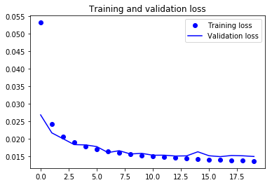
From the above plot, you can derive some intuition that the model is overfitting at some epochs while being in sync for most of the time. You can definitely try to improve the performance of the model by introducing some complexity into it so that the loss can reduce more, try training it for more epochs and then decide.

Predicting on Test dataset

pred = autoencoder.predict(x_test_noisy)

plt.figure(figsize=(20, 4))
print("Test Images")
for i in range(10,20,1):
    plt.subplot(2, 10, i+1)
    plt.imshow(test_data[i, ..., 0], cmap='gray')
    curr_lbl = test_labels[i]
    plt.title("(Label: " + str(label_dict[curr_lbl]) + ")")
plt.show()    
plt.figure(figsize=(20, 4))
print("Test Images with Noise")
for i in range(10,20,1):
    plt.subplot(2, 10, i+1)
    plt.imshow(x_test_noisy[i, ..., 0], cmap='gray')
plt.show()    

plt.figure(figsize=(20, 4))
print("Reconstruction of Noisy Test Images")
for i in range(10,20,1):
    plt.subplot(2, 10, i+1)
    plt.imshow(pred[i, ..., 0], cmap='gray')  
plt.show()

Test Images

Test Images with Noise

Reconstruction of Noisy Test Images

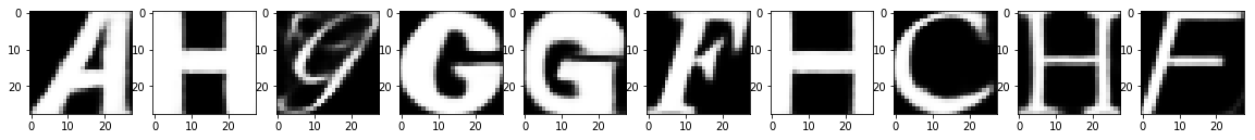
It looks like that, within just 20 epochs, a fairly simple network architecture did a pretty good job in removing the noise from the test images, isn't it?

Go Further!

This tutorial was good start to understanding autoencoders both theoretically and practically. If you were able to follow along easily or even with little more efforts, well done! Check out DataCamp's Keras Tutorial: Deep Learning in Python tutorial and Introduction to Deep Learning in Python course.

In the next tutorial, you will be learning how to read images from scratch, analyse, preprocess and feed them into the model using a fingerprint dataset. You'll also learn how to read medical images of T-1 modality and reconstruct them using an autoencoder!

There is still a lot to cover, so why not take DataCamp’s Deep Learning in Python course? If you haven’t done so already. You will learn from the basics and slowly will move into mastering the deep learning domain, it will undoubtedly be an indispensable resource when you’re learning how to work with convolutional neural networks in Python, how to detect faces, objects etc.