
Course
Feature Engineering for Machine Learning in Python
4 hr
37.6K
Even though most people associate Amazon with prime deliveries and content, the company is also top-rated among developers. Specifically, Amazon Web Services (AWS) offers cloud technologies for more than 1 million active users, including enterprise corporations and small-to-medium-sized businesses.
In this article, we will focus on AWS SageMaker , a dedicated platform for performing end-to-end machine learning (ML) workflows on a massive scale, which is part of the AWS ecosystem. By the end of this article, we will have a deployed model we can use to send requests to generate predictions for a classification task.
Amazon SageMaker is a fully managed service that provides tools and infrastructure for building, training, and deploying machine learning models. It simplifies the machine learning workflow, enabling data scientists and developers to create, train, and deploy models quickly and efficiently.
In a typical machine learning project, you will go through many stages:
Each stage requires a different set of tools and a team of skilled experts to orchestrate them seamlessly. Amazon SageMaker brings this entire process into a single platform. Here are some of its benefits:
These benefits make Amazon SageMaker a powerful and flexible platform for building, training, and deploying machine learning models at scale.
As mentioned, SageMaker is part of the AWS ecosystem, which includes many cloud computing solutions that provide storage, networking, databases, analytics, and machine learning capabilities. All these solutions work together in sync with SageMaker to unify your machine learning workflow.
For this reason, SageMaker requires you to create an AWS account if you don’t already have one.
To create your account, navigate to https://aws.amazon.com/ and follow the process to create a new account.
The sign-up process includes adding billing information and verifying your phone number. Don’t worry — you won’t be charged until you actually start using some of the SageMaker functionality (which is cost-effective, usually).
Once complete, you will be directed to your AWS console, which typically looks like the following image. Note that some of the console widgets might be different in your case.
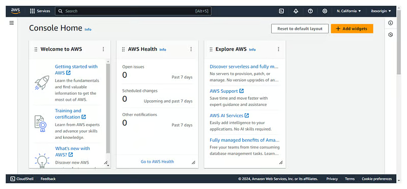
Now, we will create a JupyterLab session to execute code on Amazon’s cloud machines.
From your AWS console, search for the SageMaker dashboard using the search bar at the top of the screen:
Then, scroll down to find the “Notebooks” tab, and inside it, the “Notebooks instances” option . You will see no instances, so we need to create one:
To create a new notebook, click on the “Create notebook instance” at the top right corner of the screen. Then fill in the following fields:
sagemaker-test.Once you have filled in all the required information, click “Create notebook instance”.
When the “Pending” status changes to “inService”, you can launch JupyterLab by clicking on the “Open in JupyterLab” link next to the notebook:
As soon as the instance is in service, the clock starts ticking and the billing begins. If you decide to take a break, don’t forget to stop the instance by clicking on “Actions” and then “Stop” to prevent unnecessary costs. The idle shutdown is two hours by default:
If you stop a notebook instance, you can restart it again later. Your environment will be preserved.
In this section, we will learn how to upload a local file to Amazon’s servers, which is a requirement for SageMaker.
We will build a multi-class classifier using the Dry Bean dataset from the UCI ML repository. It contains 13k instances of beans and their 15 numeric measurements.
The task is to classify them into seven types of beans: Seker, Barbunya, Bombay, Cali, Dermosan, Horoz and Sira.

The seven types of beans: Seker, Barbunya, Bombay, Cali, Dermosan, Horoz and Sira.
After downloading, save the Excel file inside the downloaded ZIP to your local data directory in JupyerLab, and then add the following code to your notebook:
from pathlib import Path

cwd = Path.cwd()
data_path = cwd / "data" / "Dry_Bean_Dataset.xlsx"
Then, by adding the following code, we can read the Excel file with pandas and save it as a CSV:
import pandas as pd

beans = pd.read_excel(data_path)
beans.to_csv(cwd / "data" / "dry_bean.csv", index=False)Our dataset must be inside an S3 bucket for SageMaker to access it. AWS S3 is a cloud storage solution that allows you to keep project-related objects in buckets hosted on Amazon servers.
To create a bucket, follow these steps:
dry-bean-bucket like I did.
Once the bucket is created, click on it to upload the CSV file we saved before:
Afterward, you can return to the JupyterLab interface because we will finally run some code!
In this section, we will go through an end-to-end workflow that will take us from a CSV dataset to a model deployed to an endpoint. But before we get lost in the technical details, let’s take a moment to understand what we will do at a high level.
Doing machine learning in SageMaker is slightly different than doing it on your local machine. We’ve already covered the first steps:
Like your local notebooks, SageMaker notebook instances are for exploratory analysis — data cleaning, exploration, ingestion and basic experimentation.
Once you reach the model training phase, SageMaker expects you to play by its rules. Specifically, for SageMaker to deploy your custom models as endpoints, it requires a training script that does the following:
The script must also dynamically accept any variables as command-line arguments. So, anything you want to change in the future inside the script must be set as command-line arguments (model hyperparameters, file paths, etc.).
Once this script is ready, it is fed into special estimators provided by SageMaker. They are companions for popular ML libraries such as scikit-learn, XGBoost, TensorFlow, PyTorch, etc. Using these estimators, SageMaker builds Docker containers around your script, deploying it as an endpoint to serve it at scale.
All of the previous points will start to make sense as we go through them step-by-step.
Let’s start by importing the necessary libraries inside the sagemaker-test notebook you created earlier:
import boto3
import numpy as np
import pandas as pd
import sagemaker
from sagemaker import get_execution_role
from sklearn.model_selection import train_test_split
Here's what some of these imports do:
sagemaker is the official Python SDK that trains and deploys machine learning models on Amazon SageMaker. With the SDK, you can train and deploy models using popular deep learning frameworks, algorithms provided by Amazon, or your algorithms built into SageMaker-compatible Docker images.boto3 is another official Python SDK, but it serves as a bridge between your code and all AWS services, not just SageMaker. You can learn more about boto3 in this course. After the imports, let’s create some resources we will need throughout the tutorial:
sm_boto3 = boto3.client("sagemaker")
sess = sagemaker.Session()boto3. Both of these objects allow us to interact with the SageMaker platform in different ways.
Now, let’s define a few global variables we need:
region = sess.boto_session.region_name
BUCKET_URI = "s3://dry-bean-bucket"
BUCKET_NAME = "dry-bean-bucket"
DATASET_PATH = f"{BUCKET_URI}/dry_bean.csv"
TARGET_NAME = "Class"
These variables are self-explanatory and we will use them throughout the tutorial.
In most of your data projects, the training dataset will be stored in a cloud storage solution such as BigQuery, GCS, or an AWS S3 bucket. We stored ours in the last one, so let’s load it using pandas. To do that, add the following code to your notebook and execute it:
dry_bean = pd.read_csv(DATASET_PATH)
dry_bean.head()
One advantage of working in a Sagemaker notebook is that we can read files from S3 using pandas directly. All SageMaker environments are configured with your credentials to allow pandas to download the CSV from the bucket. The code wouldn’t have worked if you ran it locally.
Spending some time performing EDA (Exploratory Data Analysis) must be a part of every project you work on and this one isn’t the exception. However, we won’t be performing a deep analysis here as this will distract us from the article's main topic.
We will settle for printing a few summary statistics and charts:
dry_bean.info()<class 'pandas.core.frame.DataFrame'>
RangeIndex: 13611 entries, 0 to 13610
Data columns (total 17 columns):
# Column Non-Null Count Dtype
--- ------ -------------- -----
0 Area 13611 non-null int64
1 Perimeter 13611 non-null float64
2 MajorAxisLength 13611 non-null float64
3 MinorAxisLength 13611 non-null float64
4 AspectRation 13611 non-null float64
5 Eccentricity 13611 non-null float64
6 ConvexArea 13611 non-null int64
7 EquivDiameter 13611 non-null float64
8 Extent 13611 non-null float64
9 Solidity 13611 non-null float64
10 roundness 13611 non-null float64
11 Compactness 13611 non-null float64
12 ShapeFactor1 13611 non-null float64
13 ShapeFactor2 13611 non-null float64
14 ShapeFactor3 13611 non-null float64
15 ShapeFactor4 13611 non-null float64
16 Class 13611 non-null object
dtypes: float64(14), int64(2), object(1)
memory usage: 1.8+ MBThe information above tells us that there are 16 numeric features and a single target named Class. The dataset is small, with only 13k instances, so we won’t need powerful machines or spend a lot of money to train a model.
Next, let’s create a pair plot of a few important features using seaborn:
import seaborn as sns

sns.pairplot(
   dry_bean,
   vars=["Area", "MajorAxisLength", "MinorAxisLength", "Eccentricity", "roundness"],
   hue="Class",
);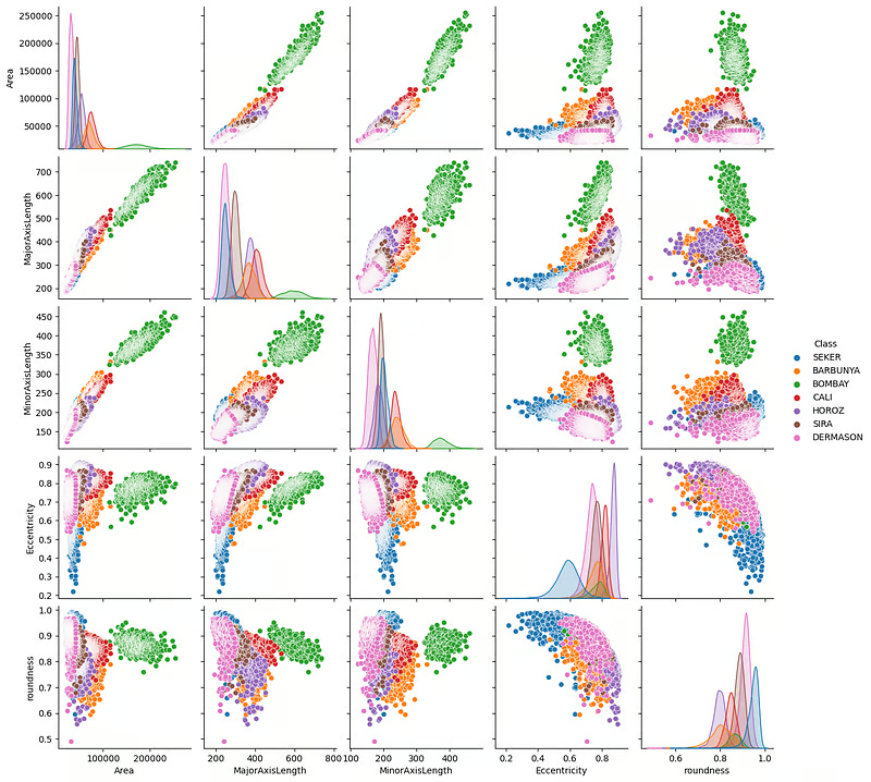
The plots above show that the beans are clearly distinct in terms of their physical measurements. The green beans (Bombay) are especially well-defined.
We can also plot a correlation matrix to see the relationship between features:
import matplotlib.pyplot as plt

correlation = dry_bean.corr(numeric_only=True)

# Create a square heatmap with center at 0
sns.heatmap(correlation, center=0, square=True, cmap="coolwarm", vmin=-1, vmax=1)
plt.show()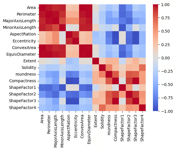
The plot shows many perfectly correlated (positive and negative) features, which makes sense since all features are related to physical measurements.
At this point, I will leave it to you to continue the exploration.
After exploration, you must address any quality or logical issues in your dataset and engineer new features if needed before training.
The Dry Bean dataset is fairly clean, so our job is easy. We only need to encode the target because it contains text. We will use scikit-learn to do this:
from sklearn.preprocessing import LabelEncoder

# For preprocessing
df = dry_bean.copy(deep=True)

# Encode the target
le = LabelEncoder()
df[TARGET_NAME] = le.fit_transform(df[TARGET_NAME])
Once preprocessing is done, we must split the dataset:
from sklearn.model_selection import train_test_split

# Split the data into two sets
train, test = train_test_split(df, random_state=1, test_size=0.2)
You can split the data further into a third validation set if you prefer, but we will keep it simple for now.
Now, let’s save the datasets as CSVs:
train.to_csv("dry-bean-train.csv")
test.to_csv("dry-bean-test.csv")
And upload them to our S3 bucket:
# Send data to S3. SageMaker will take training data from s3
trainpath = sess.upload_data(
   path="dry-bean-train.csv",
   bucket=BUCKET_NAME,
   key_prefix="sagemaker/sklearncontainer",
)

testpath = sess.upload_data(
   path="dry-bean-test.csv",
   bucket=BUCKET_NAME,
   key_prefix="sagemaker/sklearncontainer",
)
The .upload_data() function of the session object returns the full path to the uploaded file, which is stored in the trainpath and testpath variables, respectively. We will use these paths later.
In a new notebook cell, paste the following code:
%%writefile script.py

import argparse
import os
import joblib
import numpy as np
import pandas as pd
from sklearn.ensemble import RandomForestClassifier
from sklearn.metrics import balanced_accuracy_score

if __name__ == "__main__":
   print("extracting arguments")
   parser = argparse.ArgumentParser()

   # Hyperparameters sent by the client are passed as command-line arguments to the script.
   parser.add_argument("--n-estimators", type=int, default=10)
   parser.add_argument("--min-samples-leaf", type=int, default=3)

   # Data, model, and output directories
   parser.add_argument("--model-dir", type=str, default=os.environ.get("SM_MODEL_DIR"))
   parser.add_argument("--train", type=str, default=os.environ.get("SM_CHANNEL_TRAIN"))
   parser.add_argument("--test", type=str, default=os.environ.get("SM_CHANNEL_TEST"))
   parser.add_argument("--train-file", type=str, default="dry-bean-train.csv")
   parser.add_argument("--test-file", type=str, default="dry-bean-test.csv")
   args, _ = parser.parse_known_args()

   print("reading data")

   train_df = pd.read_csv(os.path.join(args.train, args.train_file))
   test_df = pd.read_csv(os.path.join(args.test, args.test_file))

   print("building training and testing datasets")

   X_train = train_df.drop("Class", axis=1)
   X_test = test_df.drop("Class", axis=1)
   y_train = train_df[["Class"]]
   y_test = test_df[["Class"]]

   # Train model
   print("training model")

   model = RandomForestClassifier(
       n_estimators=args.n_estimators,
       min_samples_leaf=args.min_samples_leaf,
       n_jobs=-1,
   )

   model.fit(X_train, y_train)

   # Print abs error
   print("validating model")

   bal_acc_train = balanced_accuracy_score(y_train, model.predict(X_train))
   bal_acc_test = balanced_accuracy_score(y_test, model.predict(X_test))

   print(f"Train balanced accuracy: {bal_acc_train:.3f}")
   print(f"Test balanced accuracy: {bal_acc_test:.3f}")

   # Persist model
   path = os.path.join(args.model_dir, "model.joblib")
   joblib.dump(model, path)
   print("model persisted at " + path)
The %%writefile script.py magic command in the above script converts the cell's contents into a Python script instead of running it.
Now, let's go through what's happening in the script step-by-step:
import argparse
import os
import joblib
import numpy as np
import pandas as pd
from sklearn.ensemble import RandomForestClassifier
from sklearn.metrics import balanced_accuracy_score
First, we import a few required libraries.
if __name__ == "__main__":
   print("extracting arguments")
   parser = argparse.ArgumentParser()

   # Hyperparameters sent by the client are passed as command-line arguments to the script.
   parser.add_argument("--n-estimators", type=int, default=10)
   parser.add_argument("--min-samples-leaf", type=int, default=3)

   # Data, model, and output directories
   parser.add_argument("--model-dir", type=str, default=os.environ.get("SM_MODEL_DIR"))
   parser.add_argument("--train", type=str, default=os.environ.get("SM_CHANNEL_TRAIN"))
   parser.add_argument("--test", type=str, default=os.environ.get("SM_CHANNEL_TEST"))
   parser.add_argument("--train-file", type=str, default="dry-bean-train.csv")
   parser.add_argument("--test-file", type=str, default="dry-bean-test.csv")
   args, _ = parser.parse_known_args()
Then, we create an argument parser object to read command-line arguments. As I mentioned, any value that may be updated in the future must be passed as CLI arguments. This section defines those arguments:
If you pay attention to the default values of the model-dir, train and test directories, you will see some environment variables. Those are taken from the SageMaker SDK docs, which also provide instructions for writing such script files.
print("reading data")
train_df = pd.read_csv(os.path.join(args.train, args.train_file))
test_df = pd.read_csv(os.path.join(args.test, args.test_file))
print("building training and testing datasets")
X_train = train_df.drop("Class", axis=1)
X_test = test_df.drop("Class", axis=1)
y_train = train_df[["Class"]]
y_test = test_df[["Class"]]
Once we define the dynamic values, we read and build the training and testing datasets. As you can see, instead of passing a hard-coded path, we are using the args.argument values.
# Train model
print("training model")

model = RandomForestClassifier(
    n_estimators=args.n_estimators,
    min_samples_leaf=args.min_samples_leaf,
    n_jobs=-1,
)

model.fit(X_train, y_train)

# Print abs error
print("validating model")

bal_acc_train = balanced_accuracy_score(y_train, model.predict(X_train))
bal_acc_test = balanced_accuracy_score(y_test, model.predict(X_test))

print(f"Train balanced accuracy: {bal_acc_train:.3f}")
print(f"Test balanced accuracy: {bal_acc_test:.3f}")
We fit the model and evaluate it on both training and test datasets and then we print the performance.
# Persist model
path = os.path.join(args.model_dir, "model.joblib")
joblib.dump(model, path)
print("model persisted at " + path)
Finally, we save the model to the model directory using joblib.
When you run this cell in your notebook, script.py file will appear in your JupyterLab environment. You can check if it is working correctly by executing it like below:
! python script.py --n-estimators 100 \

                  --min-samples-leaf 2 \

                  --model-dir ./ \

                  --train ./ \

                  --test ./ \
extracting arguments
reading data
building training and testing datasets
validating model
Train balanced accuracy: 1.000
Test balanced accuracy: 0.998
model persisted at ./modejoblibGreat, we’ve got a 99% balanced accuracy score—as good as it gets! This means we can finally start a training job.
Now, we will pass the script to a SageMaker estimator object. In the context of AWS, a training job is a process where a model is trained using a specified algorithm, dataset, and computing resources provided by AWS SageMaker. Unlike training on a local machine or notebook, this job runs in the cloud on scalable infrastructure, allowing for more computational power, faster processing, and the ability to handle larger datasets.
Add the following code on a new cell in your notebook:
# We use the Estimator from the SageMaker Python SDK
from sagemaker.sklearn.estimator import SKLearn
FRAMEWORK_VERSION = "0.23-1"

sklearn_estimator = SKLearn(
   entry_point="script.py",
   role=get_execution_role(),
   instance_count=1,
   instance_type="ml.c5.xlarge",
   framework_version=FRAMEWORK_VERSION,
   base_job_name="rf-scikit",
   hyperparameters={
       "n-estimators": 100,
       "min-samples-leaf": 3,
   },
)
In the above code, the SKLearn class deals with scikit-learn scripts. It has a few essential parameters that need explanation:
entry_point: The path to the script.role: The username that has access to SageMaker.instance_count: How many machines to spin up.instance_type: The type of the machine.For hyperparameters, only pass the ones you defined in the training script. Otherwise, there will be an error.
Now, we can fit this estimator into our data:
# Launch training job, with asynchronous call
sklearn_estimator.fit({"train": trainpath, "test": testpath}, wait=True)
If you remember from earlier sections in this tutorial, trainpath and testpath are S3 bucket paths pointing to our CSV files.
Once you run the cell with the code above, training starts:
INFO:sagemaker:Creating training-job with name: rf-scikit-2024-06-04-10-36-31-142

2024-06-04 10:36:31 Starting - Starting the training job...

2024-06-04 10:36:46 Starting - Preparing the instances for training...

2024-06-04 10:37:13 Downloading - Downloading input data...

2024-06-04 10:37:53 Training - Training image download completed. Training in progress...
SageMaker downloads the necessary Docker image that lets you run scikit-learn code and executes your script. Once it finishes, you will get the following message:
2024-06-04 10:38:17 Uploading - Uploading generated training model

2024-06-04 10:38:17 Completed - Training job completed

Training seconds: 65

Billable seconds: 65
If you go to the “SageMaker” > “Traning” > “Training Jobs” section of your SageMaker dashboard, you will also see the training job listed there.
Since our dataset is small, we got away by using a low-cost, low-configuration machine for training : ml.c5.xlarge. However, in your own projects, you may have to deal with datasets containing millions of records or massive image datasets. In those cases, you must choose machines offering significantly more power and GPUs.
Using these machines on demand can be very expensive. To cut down costs, Amazon offers Spot Training instances. With those instances, you can choose high-powered computing resources for a low price with a single caveat — the training won’t start immediately. Instead, SageMaker waits until the demand is low and the machine you requested is available.
To enable Spot Training, you have to add only a couple of lines to the last code block:
spot_sklearn_estimator = SKLearn(
   entry_point="script.py",
   role=get_execution_role(),
   instance_count=1,
   instance_type="ml.c5.xlarge",
   framework_version=FRAMEWORK_VERSION,
   base_job_name="rf-scikit",
   hyperparameters={
       "n-estimators": 100,
       "min-samples-leaf": 3,
   },
   use_spot_instances=True,
   max_wait=7200,
   max_run=3600,
)
By setting use_spot_instances to True, you make spot_sklearn_estimator use spot training. You can also set the maximum wait time for a spot instance to become available and the maximum amount of time for training to run.
The training actually starts when you call .fit() again:
# Launch training job, with asynchronous call
spot_sklearn_estimator.fit({"train": trainpath, "test": testpath}, wait=True)Using the same training script, we can produce a hyperparameter-tuned model with a similar workflow.
First, we import the IntegerParameter class from sagemaker.tuner:
from sagemaker.tuner import IntegerParameterThe IntegerParameter class allows SageMaker to define tuning ranges for parameters that accept integer values. The tuner module contains classes for other types of parameters:
CategoricalParameter: Defines hyperparameters that take on a discrete set of categorical values.ContinuousParameter: Defines tuning ranges for hyperparameters that accept continuous values.But we will stick to IntegerParameter in this tutorial since we are only tuning two parameters of Random Forest:
# We use the Hyperparameter Tuner
from sagemaker.tuner import IntegerParameter

# Define exploration boundaries
hyperparameter_ranges = {
   "n-estimators": IntegerParameter(20, 100),
   "min-samples-leaf": IntegerParameter(2, 6),
}
Then, we create a tuner object:
# Create Optimizer
Optimizer = sagemaker.tuner.HyperparameterTuner(
   estimator=sklearn_estimator,
   hyperparameter_ranges=hyperparameter_ranges,
   base_tuning_job_name="RF-tuner",
   objective_type="Maximize",
   objective_metric_name="balanced-accuracy",
   metric_definitions=[
       {"Name": "balanced-accuracy", "Regex": "Test balanced accuracy: ([0-9.]+).*$"}
   ],  # Extract tracked metric from logs with regexp
   max_jobs=10,
   max_parallel_jobs=2,
)
The Optimizer’s essential parameters are:
estimator: The estimator object, compatible with your training script.hyperparameter_ranges: The range of parameters defined with classes from tuner module.objective_type: Whether to maximize or minimize the given metric. Balanced accuracy should be maximized.metric_definitions: The name of metrics to be optimized and how they can be retrieved from training logs.The metric_definitions parameter is a bit tricky because it offers a lot of flexibility in how you define the metrics.
In the training script, we are reporting balanced accuracy using the following log message:
print(f"Train balanced accuracy: {bal_acc_train:.3f}")
print(f"Test balanced accuracy: {bal_acc_test:.3f}")
What metric_definitions asks from us is that we capture that message using regular expressions. So, we have the following dictionary, which gives a custom name to the captured metric that starts with “Test balanced accuracy”.
{
   "Name": "balanced-accuracy",
   "Regex": "Test balanced accuracy: ([0-9.]+).*$",
}
The rest of the code is familiar:
Optimizer.fit({"train": trainpath, "test": testpath})INFO:sagemaker:Creating hyperparameter tuning job with name: RF-tuner-240604-1049Once the optimizer finishes tuning, you can display its results as a DataFrame:
# Get tuner results in a df
results = Optimizer.analytics().dataframe()

while results.empty:
   time.sleep(1)
   results = Optimizer.analytics().dataframe()

results.head()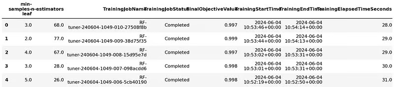
Then, you can retrieve the best estimator:
best_estimator = Optimizer.best_estimator()Once you decide which model you will use for your experiments, you can upload it to SageMaker with all its artifacts. This task can be done using boto3:
artifact_path = sm_boto3.describe_training_job(
   TrainingJobName=best_estimator.latest_training_job.name
)["ModelArtifacts"]["S3ModelArtifacts"]

print("Model artifact persisted at " + artifact)
Model artifact persisted at s3://sagemaker-us-east-1-496320894061/RF-tuner-240604-1049-009-38d75f35/output/model.tar.gzThe describe_training_job() function takes an estimator object and pushes it to a default S3 location provided by SageMaker. Above, you can see that the function converted the model into a tarball before uploading.
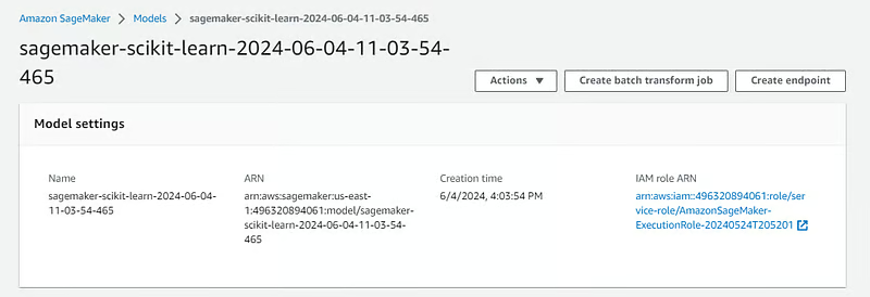
The uploaded models will be visible to you under the “Inference” > “Models” section of your SageMaker dashboard:
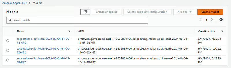
If you click on any of them, you will see a “Create endpoint” button on the top right of the screen:
You can deploy the model using that button, or you can do it with code by going back to the notebook instance and using the .deploy() method:
from sagemaker.sklearn.model import SKLearnModel

model = SKLearnModel(
   model_data=artifact_path,
   role=get_execution_role(),
   entry_point="script.py",
   framework_version=FRAMEWORK_VERSION,
)
This time, we are using the SKLearnModel class, which is used for already-trained models. It requires the S3 location where the artifacts are stored and the script used to train it. Once you provide that information, you can run the code to deploy it:
predictor = model.deploy(instance_type="ml.c5.large", initial_instance_count=1)
INFO:sagemaker:Creating model with name: sagemaker-scikit-learn-2024-06-04-11-03-54-465
INFO:sagemaker:Creating endpoint-config with name sagemaker-scikit-learn-2024-06-04-11-03-54-960
INFO:sagemaker:Creating endpoint with name sagemaker-scikit-learn-2024-06-04-11-03-54-960
Afterward, you should see the endpoint listed under “Inference” > “Endpoints” section of your SageMaker dashboard:
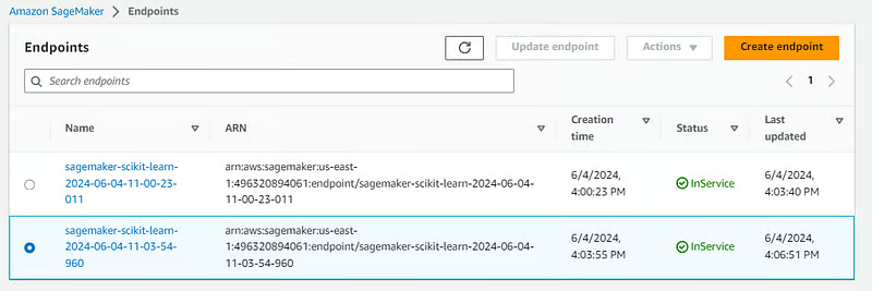
To use it for prediction, you can use the .predict() method of the endpoint object from your notebook:
preds = predictor.predict(test.sample(4).drop("Class", axis=1))
preds
array([3, 0, 1, 2])Congratulations, you just deployed your first model with SageMaker!
Once you are done using it, don’t forget to delete the endpoint, as it constantly incurs new costs:
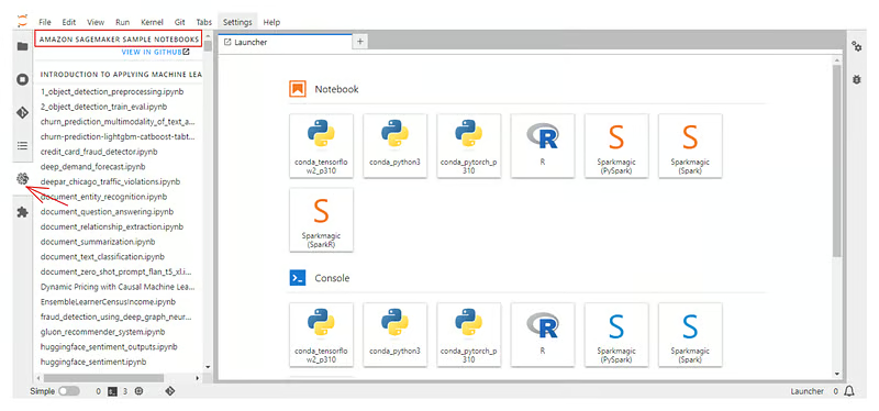
sm_boto3.delete_endpoint(EndpointName=predictor.endpoint)Don’t forget, each notebook instance you create in SageMaker comes with a separate tab with example notebooks that showcase SageMaker’s different features:
Also, check out the official documentation for SageMaker Python SDK.
Today, we have learned how to use one of the most popular enterprise machine learning platforms : AWS SageMaker. We’ve covered everything from creating an AWS account to deploying ML models as endpoints using SageMaker.
Just like with any platform, we’ve only scratched its surface. You can do so much more if you combine it with other AWS technologies in your projects. Here are some related resources to check out:
Learn more about machine learning and AWS with these courses!
Course
Course
Course
Tutorial
Joleen Bothma
Tutorial
Dan Becker
Tutorial
Moez Ali
Tutorial
DataCamp Team
Tutorial
Moez Ali
Tutorial
Zoumana Keita