Dropout Regularization Using PyTorch: A Hands-On Guide

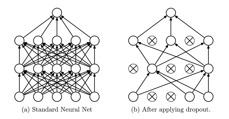
Dropout regularization is a technique used in neural networks to prevent overfitting, which occurs when a model learns the noise in the training data rather than the actual pattern. 

In 2012, Geoffrey Hinton (a Turing Award recipient) and his colleagues introduced the technique in a research paper, and it has been widely adapted to train deep learning models ever since.

This tutorial will introduce the concept of dropout regularization, reinforce why we need it, and introduce the functions that help implement it in PyTorch. You will also learn implementation details through hands-on examples, with advanced tips for effectively using dropout in your future deep learning projects.

What is Dropout Regularization, and Why Do We Need it?

The core idea of dropout is to randomly “drop out” (set to zero) a fraction of the neurons in the network during the training phase. This means that a certain percentage of neurons are ignored or “dropped out " during each forward and backward pass, making the network’s architecture dynamically different for each training batch.

Dropout regularization. (Source)

The dropout layer has become an essential layer in neural networks due to the benefits it provides:

• Preventing overfitting: Dropout randomly drops specific neurons during training, preventing the network from becoming too reliant on them. This is generally the core benefit for which we use dropout. 
• Improving generalization: Since different neurons are dropped in each training iteration, the network effectively trains multiple sub-networks. This ensemble-like behavior enhances the model's generalization ability.
• Reducing co-adaptation: Neurons in a network can co-adapt, meaning they develop dependencies on each other. Dropout reduces these dependencies by ensuring each neuron operates more independently, improving the network’s ability to learn valuable features.

Since we understand the concept of dropout, let’s dive into the implementation of it.

Understanding the Dropout Layer in PyTorch

Popular deep learning libraries such as Tensorflow and PyTorch have provided simplified modules and functions, so implementing dropout regularization in neural network models is straightforward. 

As the title suggests, this tutorial is focused on implementing dropout regularization using PyTorch, but if you choose to do it in Tensorflow, the instructions are available in the Tensorflow official documentation. 

PyTorch is an open-source machine learning library developed by Facebook’s (now Meta) AI Research Lab (FAIR), which is widely used for deep learning and artificial intelligence applications. In PyTorch, dropout can be implemented using the torch.nn.Dropout Class.

The torch.nn.Dropout Class

The syntax of the torch.nn.Dropout Class is as follows:

torch.nn.Dropout(p=0.5, inplace=False)

Where:

• p is the probability of an element to be zeroed. The default is 0.5.
• inplace: if set to True, this operation will be in place. The default is False.

In this function, during training, the Dropout layer randomly zeroes some elements of the input tensor with probability p. The zeroed elements are chosen independently for each forward call and are sampled from a Bernoulli distribution. Each channel is zeroed out independently on every forward call. 

During evaluation, the dropout layer is turned off, meaning the layer computes an identity function. This ensures that all neurons are active and no scaling is applied.

Since we have understood how dropout regularization works and the function used in PyTorch, let’s bring it together through a hands-on example next.

Hands-on Example: Building a Neural Network Model with Dropout Regularization

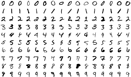
We will take the popular MNIST dataset and build a simple convolutional neural network to detect handwritten numbers from images. We’ll then learn to add dropout layers to the neural network and examine its impact.

The environment setup

First, if you haven’t installed Python, the installation instructions can be found on the official Python website. Once Python is installed, you can use the package manager pip to install the PyTorch libraries. 

Open your terminal and run the following command:

pip install torch torchvision

Please note that the PyTorch libraries depend on your environment and CUDA version. The official installation documentation provides clear installation instructions based on your environment setting.

If you’re hurrying to test the codes and prefer to skip the environment setup, you could open a new Google Collab notebook with PyTorch pre-installed to go hands-on immediately.

The MNIST dataset

Since the MNIST (Modified National Institute of Standards and Technology) dataset is directly available in the PyTorch library, we don’t have to download it elsewhere.

The MNIST dataset is a large collection of handwritten digits commonly used for training and testing. It consists of 70,000 grayscale images of digits (0–9), divided into 60,000 training images and 10,000 testing images. Each image is labeled with the digit it represents, making it a supervised learning dataset.

The MNIST dataset.

We shall load the relevant libraries and read the dataset.

import torch
import torch.nn as nn
import torch.optim as optim
import torchvision
import torchvision.transforms as transforms
from torch.utils.data import DataLoader, random_split
import matplotlib.pyplot as plt

# Transformation to normalize the data
transform = transforms.Compose([
    transforms.ToTensor(),
    transforms.Normalize((0.5,), (0.5,))
])

# Loading the MNIST dataset
full_dataset = torchvision.datasets.MNIST(root='./data', train=True, download=True, transform=transform)
test_dataset = torchvision.datasets.MNIST(root='./data', train=False, download=True, transform=transform)

# Splitting the dataset into training and validation sets
train_size = int(0.8 * len(full_dataset))
val_size = len(full_dataset) - train_size
train_dataset, val_dataset = random_split(full_dataset, [train_size, val_size])

train_loader = DataLoader(dataset=train_dataset, batch_size=100, shuffle=True)
val_loader = DataLoader(dataset=val_dataset, batch_size=100, shuffle=False)
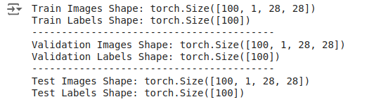
test_loader = DataLoader(dataset=test_dataset, batch_size=100, shuffle=False)

For this example, 20% of the training images have been split into validation images. Next, we check the dimensions of the datasets:

# Inspecting the train dataset
train_data_iter = iter(train_loader)
train_images, train_labels = next(train_data_iter) 
print(f"Train Images Shape: {train_images.shape}")
print(f"Train Labels Shape: {train_labels.shape}")
print("-----------------------------------------")

# Inspecting the val dataset
val_data_iter = iter(val_loader)
val_images, val_labels = next(val_data_iter) 
print(f"Validation Images Shape: {val_images.shape}")
print(f"Validation Labels Shape: {val_labels.shape}")
print("-----------------------------------------")

# Inspecting the test dataset
test_data_iter = iter(test_loader)
test_images, test_labels = next(test_data_iter) 
print(f"Test Images Shape: {test_images.shape}")
print(f"Test Labels Shape: {test_labels.shape}")

We see the output as follows:

Output: The dimensions of the dataset.

These outputs indicate that the batches contain 100 images, each with one channel and dimensions of 28x28 pixels. The labels are simply a 1D tensor of size 100, corresponding to the labels for each image in the batch.

Defining the model without dropout

Once we have loaded and transformed the data, we define a simple convolutional neural network model, the first being the model that does not use dropout.

# Define the CNN Without Dropout
class CNNWithoutDropout(nn.Module):
   def __init__(self):
       super(CNNWithoutDropout, self).__init__()
       self.conv1 = nn.Conv2d(1, 32, kernel_size=3, stride=1, padding=1)
       self.conv2 = nn.Conv2d(32, 64, kernel_size=3, stride=1, padding=1)
       self.pool = nn.MaxPool2d(kernel_size=2, stride=2, padding=0)
       self.fc1 = nn.Linear(64 * 7 * 7, 128)
       self.fc2 = nn.Linear(128, 10)

   def forward(self, x):
       x = self.pool(torch.relu(self.conv1(x)))
       x = self.pool(torch.relu(self.conv2(x)))
       x = x.view(-1, 64 * 7 * 7)
       x = torch.relu(self.fc1(x))
       x = self.fc2(x)
       return x

model_without_dropout = CNNWithoutDropout()

After the model definition, we define the optimizer and the loss function.

criterion = nn.CrossEntropyLoss()
optimizer_without_dropout = optim.SGD(model_without_dropout.parameters(), lr=0.01, momentum=0.9)

Training the baseline model

Next, we train the model without dropout, recording the training and validation metrics. Let's write the codes as functions so that we can reuse them later.

def train_validate_model(model, train_loader, val_loader, criterion, optimizer, num_epochs=10):
   train_losses = []
   val_losses = []
   train_accuracies = []
   val_accuracies = []

   for epoch in range(num_epochs):
       model.train()
       running_loss = 0.0
       correct = 0
       total = 0

       for images, labels in train_loader:
           outputs = model(images)
           loss = criterion(outputs, labels)

           optimizer.zero_grad()
           loss.backward()
           optimizer.step()

           running_loss += loss.item()
           _, predicted = torch.max(outputs.data, 1)
           total += labels.size(0)
           correct += (predicted == labels).sum().item()

       epoch_loss = running_loss / len(train_loader)
       epoch_accuracy = 100 * correct / total
       train_losses.append(epoch_loss)
       train_accuracies.append(epoch_accuracy)

       # Validation Phase
       model.eval()
       val_loss = 0.0
       correct = 0
       total = 0

       with torch.no_grad():
           for images, labels in val_loader:
               outputs = model(images)
               loss = criterion(outputs, labels)
               val_loss += loss.item()
               _, predicted = torch.max(outputs.data, 1)
               total += labels.size(0)
               correct += (predicted == labels).sum().item()

       val_loss /= len(val_loader)
       val_accuracy = 100 * correct / total
       val_losses.append(val_loss)
       val_accuracies.append(val_accuracy)

       print(f'Epoch [{epoch+1}/{num_epochs}], Loss: {epoch_loss:.4f}, Accuracy: {epoch_accuracy:.2f}%, Val Loss: {val_loss:.4f}, Val Accuracy: {val_accuracy:.2f}%')
   return train_losses, val_losses, train_accuracies, val_accuracies

We can now call this function with the train and validation datasets.

train_losses_without_dropout, val_losses_without_dropout, train_accuracies_without_dropout, val_accuracies_without_dropout = train_validate_model(
   model_without_dropout, train_loader, val_loader, criterion, optimizer_without_dropout
)

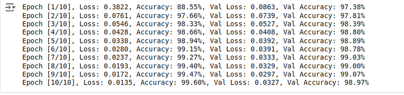
You’ll see the training and validation metrics below:

Output: Training and validation metrics.

The validation accuracy is slightly lower than the training accuracy. Even without dropout, the model performs exceptionally well during the training and validation phase, demonstrating high accuracy on both the training and validation sets.

Evaluating the baseline model

Once the training is complete, we can evaluate how the model performs in the test images to obtain the test accuracy score, which serves as our baseline score before we add dropout layers.

def evaluate_model(model, test_loader, criterion):
   model.eval()
   correct = 0
   total = 0

   with torch.no_grad():
       for images, labels in test_loader:
           outputs = model(images)
           _, predicted = torch.max(outputs.data, 1)
           total += labels.size(0)
           correct += (predicted == labels).sum().item()

   accuracy = 100 * correct / total
   return accuracy

accuracy_without_dropout = evaluate_model(model_without_dropout, test_loader, criterion)
print(f'Accuracy of the model without dropout on the test images: {accuracy_without_dropout:.2f}%')

The resulting final accuracy, as we see, is:

Output: Accuracy on the test images.

99.07% accuracy is extremely good, slightly lower than the training accuracy but better than the validation accuracy. Let's see how the model behaves when we add dropout layers, which make it harder to learn handwritten digits.

Model definition with dropout

We now understand how to define, train, and evaluate a simple neural network. Let’s repeat the procedure, starting with a model definition and adding a dropout layer.

# Define the CNN With Dropout
class CNNWithDropout(nn.Module):
   def __init__(self):
       super(CNNWithDropout, self).__init__()
       self.conv1 = nn.Conv2d(1, 32, kernel_size=3, stride=1, padding=1)
       self.conv2 = nn.Conv2d(32, 64, kernel_size=3, stride=1, padding=1)
       self.pool = nn.MaxPool2d(kernel_size=2, stride=2, padding=0)
       self.dropout = nn.Dropout(p=0.5)  # Dropout layer with 50% probability
       self.fc1 = nn.Linear(64 * 7 * 7, 128)
       self.fc2 = nn.Linear(128, 10)

   def forward(self, x):
       x = self.pool(torch.relu(self.conv1(x)))
       x = self.pool(torch.relu(self.conv2(x)))
       x = x.view(-1, 64 * 7 * 7)
       x = self.dropout(torch.relu(self.fc1(x)))  # Apply dropout after ReLU activation
       x = self.fc2(x)
       return x

model_with_dropout = CNNWithDropout()

Notice the code change: Two new lines of code have been added, which adds the dropout layers to the model definition. Yes, adding dropout layers is as simple as a few lines of code using the relevant function available in PyTorch.

We keep our loss function and the optimizer the same as the baseline model.

criterion = nn.CrossEntropyLoss()
optimizer_with_dropout = optim.SGD(model_with_dropout.parameters(), lr=0.01, momentum=0.9)

Training the model with dropout

Next, we train the model with dropout by reusing the previously written functions and recording the training and validation metrics.

train_losses_with_dropout, val_losses_with_dropout, train_accuracies_with_dropout, val_accuracies_with_dropout = train_validate_model(
   model_with_dropout, train_loader, val_loader, criterion, optimizer_with_dropout
)

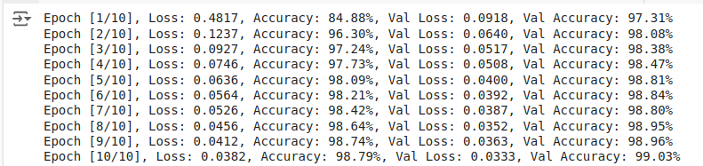
The resulting training and validation scores are:

Output: Training and validation metrics.

Compared with the model with dropout, the model without dropout achieves higher training accuracy and lower training loss, which is expected since dropout introduces noise during training, making it harder for the model to fit the training data perfectly. 

Despite the reduction in training scores, the validation accuracy of the model with dropout has increased.

Evaluating the model with dropout

During evaluation phases (including validation), dropout layers are deactivated. This means that all units are active, and no inputs are dropped.

In PyTorch, switching between training and evaluation modes is done using model.train() and model.eval(), respectively:

• model.train(): Sets the model to training mode, activating dropout and other training-specific behaviors like batch normalization.
• model.eval(): Sets the model to evaluation mode, deactivating dropout and using the full network for predictions.

Let’s calculate the test accuracy:

accuracy_with_dropout = evaluate_model(model_with_dropout, test_loader, criterion)
print(f'Accuracy of the model with dropout on the test images: {accuracy_with_dropout:.2f}%')

The resulting accuracy is as follows:

Output: Accuracy on the test images.

We get an accuracy of 99.12%, slightly better than what we got with the model without dropout. 

Comparing the effect of dropout in neural networks

Since we have stored all the metrics during our training, validation, and evaluation phases, let’s plot them into graphs using Matplotlib to analyze them better.

The code to do so is as follows:

# Plotting the Results
plt.figure(figsize=(14, 10))

# Plot training loss
plt.subplot(2, 2, 1)
plt.plot(train_losses_without_dropout, label='Without Dropout')
plt.plot(train_losses_with_dropout, label='With Dropout')
plt.title('Training Loss')
plt.xlabel('Epoch')
plt.ylabel('Loss')
plt.legend()

# Plot validation loss
plt.subplot(2, 2, 2)
plt.plot(val_losses_without_dropout, label='Without Dropout')
plt.plot(val_losses_with_dropout, label='With Dropout')
plt.title('Validation Loss')
plt.xlabel('Epoch')
plt.ylabel('Loss')
plt.legend()

# Plot training accuracy
plt.subplot(2, 2, 3)
plt.plot(train_accuracies_without_dropout, label='Without Dropout')
plt.plot(train_accuracies_with_dropout, label='With Dropout')
plt.title('Training Accuracy')
plt.xlabel('Epoch')
plt.ylabel('Accuracy (%)')
plt.legend()

# Plot validation accuracy
plt.subplot(2, 2, 4)
plt.plot(val_accuracies_without_dropout, label='Without Dropout')
plt.plot(val_accuracies_with_dropout, label='With Dropout')
plt.title('Validation Accuracy')
plt.xlabel('Epoch')
plt.ylabel('Accuracy (%)')
plt.legend()

plt.tight_layout()
plt.show()

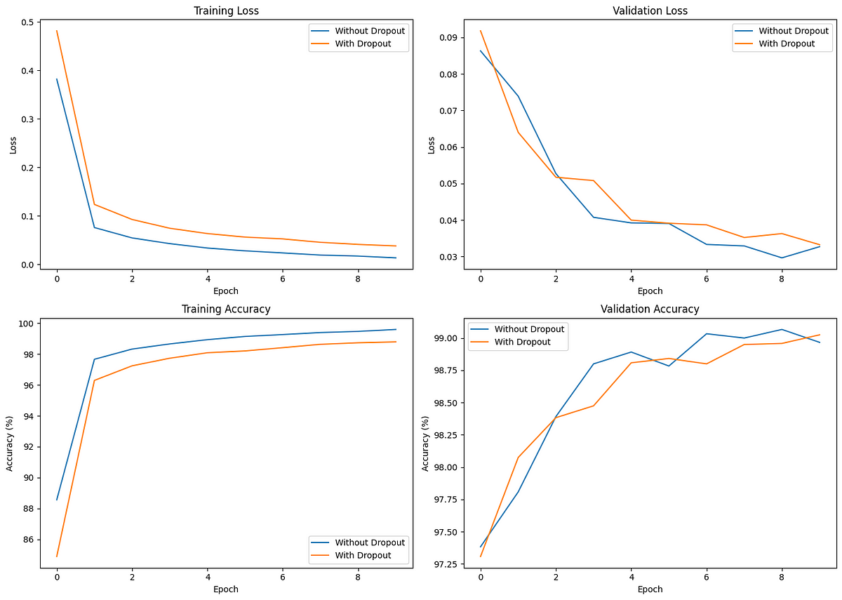
The comparison plots are as follows:

Comparing the effect of dropout on training and validation.

The initial training loss is lower for the model without dropout, indicating faster convergence. However, the model with dropout demonstrates more consistent validation loss and accuracy, indicating better generalization. 

When analyzing these plots, the model with dropout achieves a slightly higher validation accuracy (and test accuracy) than the model without dropout, despite the model with dropout having a lower training accuracy compared to the model without dropout.

Dropout helps prevent overfitting, as seen from the smaller gap between training and validation performance. Though insignificant in our example, the difference becomes increasingly crucial when training more complex and larger models.

Advanced Tips for Effective Usage of Dropout Regularization

Here are some helpful tips when you’re training deep learning models using Dropout:

• Addressing your model's core issue first: Dropout helps fight overfitting in models and improves generalization. If your model is underperforming or underfitting, it’s best to address that first by changing the algorithms, optimizing the hyper-parameters, and later turning to dropout regularization if/when overfitting occurs.
• Finding the optimal dropout rates: Never settle with a single pre-defined dropout rate because the underlying data you may be using may differ from what we used in this tutorial or what the researchers have found. It’s a good rule of thumb to run multiple experiments with dropout rates between 20% and 50% and analyze the results to find the optimal dropout rate.
• Layer-dependant dropout rates: You can apply dropout to all (or multiple) layers rather than just one hidden layer for better generalization performance. For input units, a dropout rate of 20% and a dropout rate of 50% for hidden units were found to be effective.
• Train the models for substantial epochs: Adding dropout layers makes learning patterns harder, requiring more extended training epochs than usual. 

If you’re a deep-learning practitioner, it’s worth reading the original research paper “Improving Neural Networks by Preventing Co-adaptation of Feature Detectors.” In it, the authors discuss several additional helpful guidelines based on their experiments.

Conclusion

Overfitting the training data is a common issue in neural networks, especially on larger models trained for higher iterations. Regularization techniques, such as dropout, prevent neural networks from memorizing the training data and help them better learn the useful patterns in the data.

This tutorial introduced the concept of dropout regularization, explained why we need it, and implemented it using PyTorch through an example use case. We also learned some advanced best practices and tips for using dropout effectively in deep neural networks.

To learn more about using PyTorch for deep learning tasks, check out the beginner-friendly Introduction to Deep Learning with PyTorch course and the Intermediate Deep Learning with PyTorch course, in that order.