Quantization for Large Language Models (LLMs): Reduce AI Model Sizes Efficiently

Have you ever dreamed of running your own ChatGPT directly on your laptop?

With the rapid advancements in Large Language Models (LLMs), the possibility of bringing those powerful models to consumer hardware is becoming a reality.

The key to unlocking this potential lies in quantization, a technique that allows reducing the size of these increasingly large models to run on everyday devices with minimal performance degradation — if implemented correctly!

In this guide, we will delve into the concept of quantization, explaining how it works, and the different possibilities for quantizing LLMs. Finally, we will quantize our model in two simple steps using Hugging Face’s Quanto library.

Let’s dive deep! You can follow along using the DataCamp DataLab.

The Increasing Growth of Large Language Models

As LLMs have evolved, their complexity has grown exponentially, leading to a significant increase in their number of parameters. For instance, the first GPT model, launched in 2018, had 0.11 billion parameters. By late 2019, GPT-2 expanded this to 1.5 billion, and GPT-3, released in late 2020, skyrocketed to 175 billion parameters. 

Today, GPT-4 boasts over 1 trillion parameters. This big increase presents a challenge: as models grow, so do their memory requirements, often surpassing the capacity of advanced hardware accelerators such as GPUs.

This growing demand for memory limits both the training and hosting of the models for inference, consequently restricting the accessibility and adoption of LLM-based solutions.

This growth leads to a pressing need to make these models more accessible by reducing their size. By changing the precision of some components of the model, quantization reduces the model’s memory footprint while maintaining similar performance levels.

What is Quantization?

Quantization is a model compression technique that converts the weights and activations within a large language model from high-precision values to lower-precision ones. This means changing data from a type that can hold more information to one that holds less. A typical example is converting data from a 32-bit floating-point number to an 8-bit integer.

Reducing the number of bits required for each of the model’s weights or activations leads to a significant decrease in its overall size. Consequently, quantization shrinks LLMs to consume less memory, require less storage space, and make them more energy-efficient.

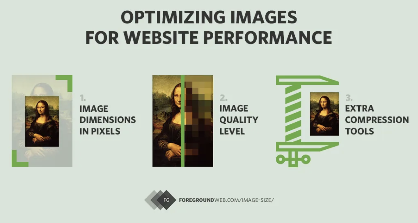
An effective analogy for understanding quantization is image compression. High-resolution images are often compressed for use on websites. This involves reducing the size of the image by removing some data or bits of information. While this typically lowers the image quality to some extent, it also decreases the image dimensions and file size, making web pages load faster while still providing a satisfactory visual experience.

Schema of image compression for faster loading in applications such as webpages.

Similarly, quantizing an LLM reduces its computational requirements, allowing it to run on less powerful hardware while still delivering adequate performance. Compressed images are easier to handle, just as quantized models are more deployable across various platforms, though there is a slight trade-off in detail or precision. As we will see, the quantization process also introduces some noise.

Theory of Quantization

Quantization is normally applied to the weights of a large language model, although it can also be applied to the activations. Model weights are parameters in a neural network that determine the strength of connections between neurons across different layers. Weights are essentially the learned coefficients that transform input data as it passes through the network.

Weights are initially set to random, meaningless values and adjusted during training based on the error between the predicted output and the actual targets. This adjustment process is guided by optimization algorithms such as gradient descent.

If you want to know more about the internals of LLMs, the course Developing Large Language Models is for you!

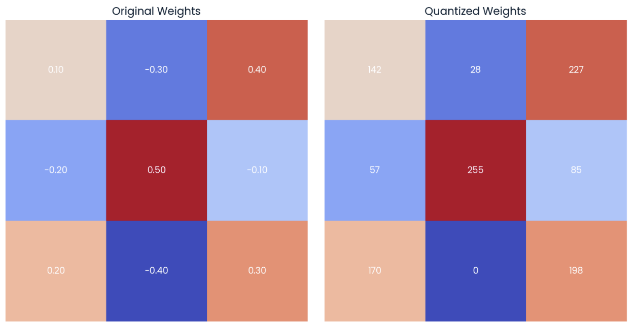
One option for quantizing a model is reducing the precision of its model weights. To illustrate that, let’s focus on the matrix on the left in the image below, which represents a 3x3 matrix of weights with four-decimal precision:

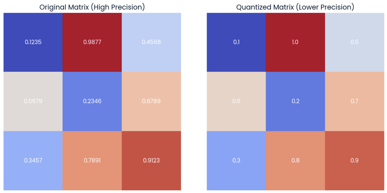
Example of a random matrix of weights with four-decimal precision (left) with its quantized form (right) by applying rounding to one-decimal precision.

On the matrix on the right, we can observe the quantized version of the original matrix. This “quantized” matrix is computed by rounding the elements of the original matrix to one decimal.

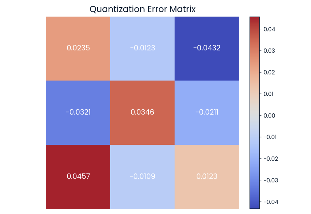
We can observe that the matrices above are not completely equal but are very similar. The value-by-value difference is known as quantization error, which we can also represent in matrix form:

Quantization error in matrix from. The darker the color, the higher the error.

Current research in quantization is focused on trying to reduce this difference as much as possible to avoid any performance degradation.

In this simple example, we are just rounding the matrix elements. In practice, quantization is performed by converting numerical values to a different data type, e.g., from a data type of higher precision to a lower precision one. For example, the default storing data type for most of the models is float32. 

In this case, we would need to allocate 4 bytes per parameter (4 times 8-bit precision). Therefore, for a 3x3 matrix like the one in the example, the total memory footprint of this matrix is 36 bytes.

By changing the data type — also known as downcasting — to int8, we would only need one byte per parameter. Therefore, the total memory footprint of the matrix turns into 9 bytes.

Brain floating point — BF16

The selected data type for the model’s weights determines how much we can reduce the model. Traditional floating-point types, like float32 and float16, have been the standard in many machine learning applications, providing a balance between accuracy and computational efficiency. Specifically, while float32 offers high precision and a wide dynamic range, it requires more memory and computational power. On the contrary, float16 offers reduced precision and range, significantly speeding up computations.

• In 2018, Google recognized the need for a floating-point format that could offer a midpoint between float32’s wide dynamic range and float16’s efficiency. 

This led to the creation of the so-called Brain Floating Point  (bfloat16), which retains the dynamic range of float32 but with reduced precision.

Downcasting

Downcasting is the formal term for converting a higher-precision data type to a lower-precision data type. By using downcasting, we reduce the memory footprint and increase speed since computations using lower precision also require less memory.

In this section, we will explore how downcasting works from float32— the default storage data type for most models — to Google’s bfloat16, and we will observe how it typically results in some loss of data.

Let’s start by defining a random tensor in PyTorch with elements of type float32 and displaying the first five elements:

import torch
# random pytorch tensor: float32, size=1000
tensor_fp32 = torch.rand(1000, dtype = torch.float32)
print(tensor_fp32[:5])
>> tensor([0.2257, 0.0480, 0.8520, 0.3115, 0.1373])

We can now downcast the tensor to bfloat16 by using the .to(dtype) method and observe the first 5 new elements:

# downcast the tensor to bfloat16 using the "to" method
tensor_fp32_to_bf16 = tensor_fp32.to(dtype = torch.bfloat16)
print(tensor_fp32_to_bf16[:5])
>> tensor([0.2256, 0.0481, 0.8516, 0.3105, 0.1377], dtype=torch.bfloat16)

As we can see, the values are quite close, although not the same. The difference becomes more noticeable when we start performing operations on the values. For example, when multiplying the original tensor by itself:

# tensor_fp32 x tensor_fp32
m_float32 = torch.dot(tensor_fp32, tensor_fp32)
print(m_float32)
>> tensor(322.1082)

If we perform the same computation with the quantized tensor, we see that the difference is higher:

# tensor_fp32_to_bf16 x tensor_fp32_to_bf16
m_bfloat16 = torch.dot(tensor_fp32_to_bf16, tensor_fp32_to_bf16)
print(m_bfloat16)
>> tensor(256., dtype=torch.bfloat16)

We can observe a clear difference between the final results due to error propagation. 

The same effect of error propagation when operating with quantized tensors occurs when downcasting LLMs, leading to a loss of information. As we have seen, using less memory implies the computation could be less precise. The effect of multiplication is similar to the real error propagation layer by layer, which accumulates and eventually affects some token predictions. 

With downcasting, performance stays acceptable when using the bfloat16 type, but it doesn’t hold for smaller data types.

Downcasting is not commonly used as an effective quantization technique due to this restriction on the data types. Instead, other methods that maintain performance closer to the original model by converting back to float32 during inference are used.

Types of Quantization

There are several types of quantization, and we’ve described each in detail below: 

Linear quantization

Linear quantization is one of the most popular quantization schemas for LLMs. In simple terms, it involves mapping the range of floating-point values of the original weights to a range of fixed-point values evenly, using the high-precision data type for inference.

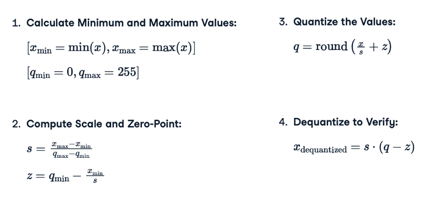
To make it as simple as possible, let’s review the steps required to apply linear quantization to a model. Note that the actual formulas are shown in the image below:

1. Calculate the minimum and maximum values: For each tensor, we need to get the minimum and maximum values to define the range of the floating-point values to quantize. The data type we want to convert to will give the minimum and maximum of the quantized range. For example, in the case of an unsigned integer, the range would be from 0 to 255 for 8-bit.
2. Compute the scale (s) and the zero-point (s) values: The scale adjusts the range of floating-point values to fit within the integer range. The zero-point ensures that zero in the floating-point range is accurately represented by an integer, maintaining numerical accuracy and stability, especially for values close to zero.
3. Quantize the values (q): This step involves mapping floating-point values to a lower precision integer range using a scale factor s and a zero point s computed in the previous step. The rounding operation ensures that the final result is a discrete integer, suitable for storage and computation in lower precision formats.
4. Dequantize: During inference, the dequantized values are used for calculations to achieve higher precision, although only the quantized weights are stored. This step will also allow you to compute the quantization error.

Let’s associate each of the steps described above with their corresponding formula:

Quantization equations used to apply linear quantization to any matrix of weights.

Is it difficult to imagine how to apply these formulas? Let’s get hands-on!

If we apply these formulas to the 3x3 weight tensor on the left in the image below, we will get the quantized matrix shown on the right. I recommend taking a few minutes to compute the maximum and minimum values of the quantized range and some of the quantized values:

Example of a random matrix of weights with two-decimal precision (left) with its quantized form (right) to int8 data type.

We can see that the lower bound of the int8 value corresponds to the lower value of the original tensor (-0.40 → 0), while the upper bound corresponds to the higher value of the original tensor (0.50 → 255). 

If we now dequantize the values using formula (4), we can see that the dequantized values are close to the original values (matrix on the left). We can compute the quantization error by calculating the point-by-point difference (matrix on the right):

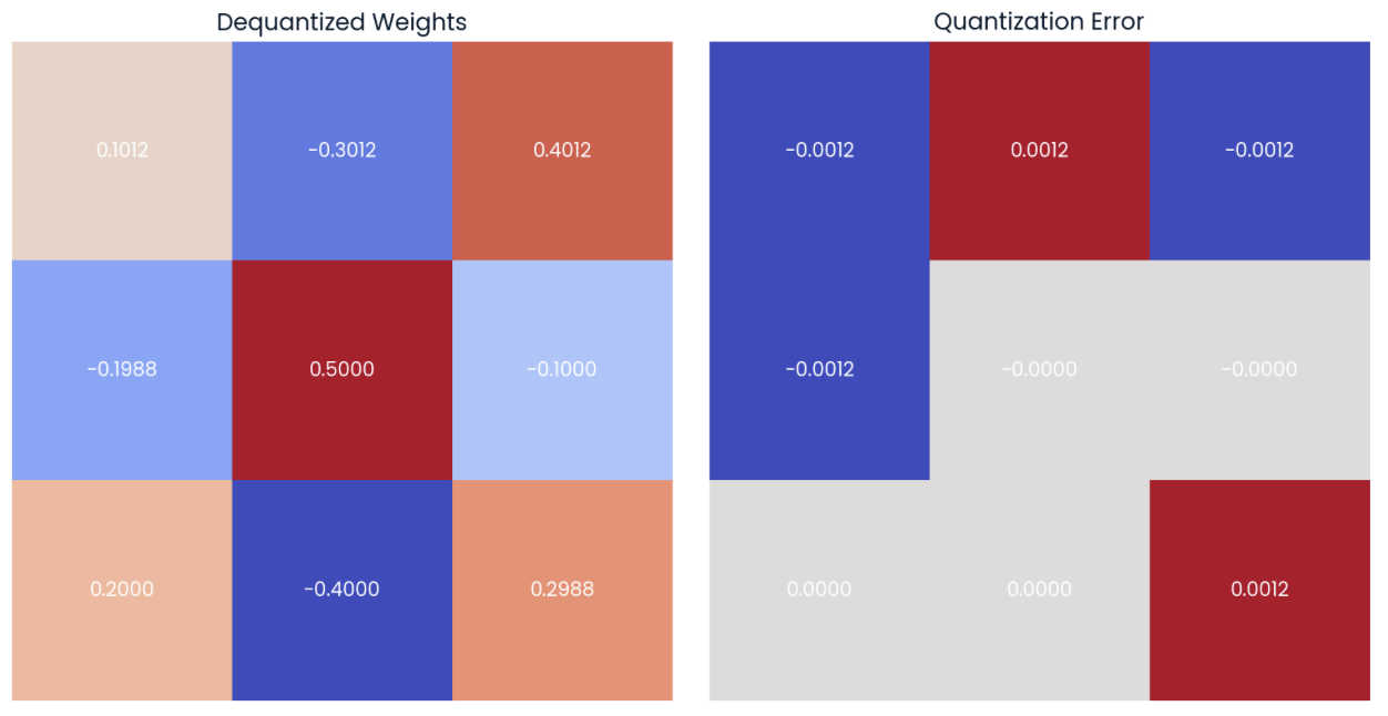
Values can be dequantized by using the quantized weights and the scale and zero-point values (left). The point-by-point difference or quantization error can be computed (right).

Linear quantization reduces the model size by storing only the quantized weights and the scale and zero-point values in memory, while using them to compute the original weights for inference and maintain the performance.

Blockwise quantization

Linear quantization is a popular option due to its simplicity, but there are multiple ways of building a mapping. Another method that is quite popular nowadays is Blockwise quantization, which is more accurate than linear quantization for models with non-uniform weight distributions.

Blockwise quantization is a more sophisticated method that involves quantizing weights in smaller blocks rather than across the entire range. This method relies on two key concepts:

1. Blockwise quantization: Weights are divided into smaller blocks, and quantization is applied to each block separately. This allows for better handling of variations within different parts of the model.
2. Distribution-aware blocks: The quantization process takes into account the relative frequency of the weights within each block, creating blocks that are aware of the distribution of the weights. This results in a more efficient mapping of values.

Weight quantization vs activation quantization

During our matrix examples, we have mainly focused on the process of quantizing the weights of a model. While weight quantization is a crucial step for model optimization, it is also important to consider that the activations of a model can be also quantized.

Activation quantization refers to the process of reducing the precision of the intermediate outputs of each layer in the network. Unlike weights, which are static (constant) once the model is trained, activations are dynamic. This means that activations change with each input to the network, making their range harder to predict.

In general, activation quantization is harder to implement than weight quantization. It requires careful calibration to ensure that the dynamic range of activations is well captured.

Weight quantization and activation quantization are complementary techniques. By applying both techniques, we can enable significant improvements in model size without compromising performance too much.

Post-Training Quantization (PTQ) vs Quantization-Aware Training (QAT)

Quantization can also be performed at different points in time. If we take a pre-trained model and quantize the model parameters during the inference phase, we are performing Post-Training Quantization (PTQ). 

This method does not involve any changes to the training process itself. The dynamic range of parameters is recalculated at runtime, similar to how we worked with the example matrices.

On the other hand, there is also the option of applying Quantization-Aware Training (QAT). This approach involves modifying the training process to simulate the effects of quantization during training. The model is trained to be robust to quantization noise, resulting in better accuracy.

During QAT, the intermediate states of the training hold both a quantized version of the weights and the original unquantized weights (also in memory!). Therefore, we use the quantized version of the model for inference, but the unquantized version of the model weights will be updated during backpropagation.

As expected, although more complex and time-consuming, QAT generally results in higher accuracy compared to PTQ.

Calibration Techniques

Some quantization methods require a calibration step. For example, we must determine the original activation range of a model before quantization. General calibration usually involves running inference on a representative dataset to optimize the quantization parameters and minimize quantization error.

During this calibration process, the quantization algorithm collects statistics about the distribution and range of the model’s activations and weights. These statistics help determine the best quantization parameters. Computing the scale and the zero-point when quantizing the weights is also a sort of calibration, but there are other types:

• Percentile calibration: Focuses on a specified percentile range of the weights, ignoring extreme outliers leading to a more robust quantization.
• Mean and standard deviation calibration: Defines the quantization range based on the statistical measures of the mean and standard deviation of the weights.

However, quantization methods like QLoRA can be used without any calibration step. 

These methods typically replace all linear layers in the model with quantized linear layers (QLinear). QLinear layers are designed to handle quantization internally, thereby eliminating the need for an additional calibration step. This makes the quantization process more straightforward to implement while still maintaining the model’s performance.

Tools for Quantization

Several tools and libraries in Python support quantization, providing tools for both PTQ and QAT. For example, pytorch and tensorflow provide quantization methods, although integrating quantization seamlessly in existing models requires a deep understanding of the libraries and model internals. See quantization options in the official PyTorch documentation. 

If you are interested in learning those powerful frameworks, I recommend the course Deep Learning in Python.

My favorite option to implement quantization in easy steps so far is the Quanto library by Hugging Face, which is designed to simplify the quantization process for PyTorch models.

Practical Steps for Quantizing a Model

A typical quantization workflow using the Quanto library by Hugging Face would consist of the following steps:

1. Select and load a pre-trained model and its corresponding tokenizer. In this case, we are going to use the Pythia 410M model from EuletherAI:

from transformers import AutoModelForCausalLM, AutoTokenizer
model_name = "EleutherAI/pythia-410m"
model = AutoModelForCausalLM.from_pretrained(model_name, 
low_cpu_mem_usage=True)
tokenizer = AutoTokenizer.from_pretrained(model_name)

The model.gpt_neox method can help in visualizing the different layers of the loaded model:

print(model.gpt_neox)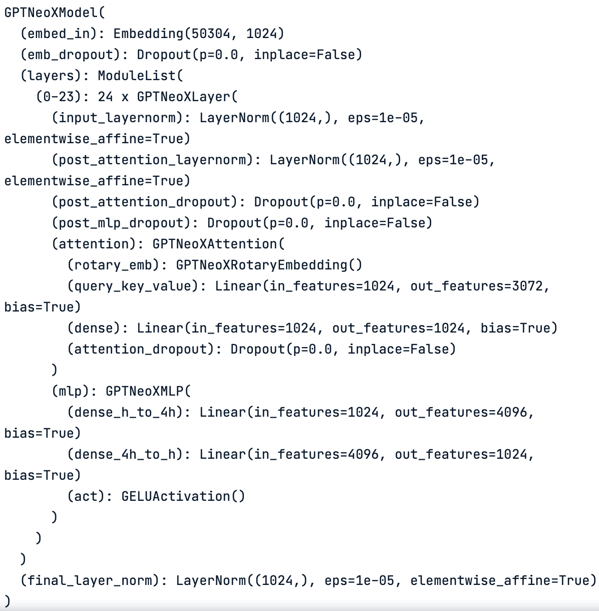

Layer-by-layer schema of the original model. The model is made of different types of layers such as linear layers and normalization layers.

We can check that the model works properly by running some test inferences. For example,

text = "Once upon a time, there was a"
inputs = tokenizer(text, return_tensors="pt")
outputs = model.generate(**inputs, max_new_tokens=10)
print(tokenizer.decode(outputs[0], skip_special_tokens=True))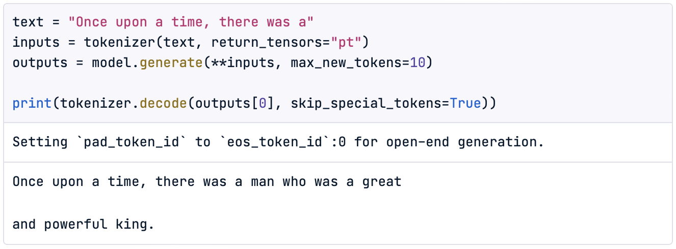

In addition, since quantizing the model will allow us to reduce its size, it is also interesting to check the original model size before starting the process:

import torch
module_sizes = compute_module_sizes(model)
print(f"The model size is {module_sizes[''] * 1e-9} GB")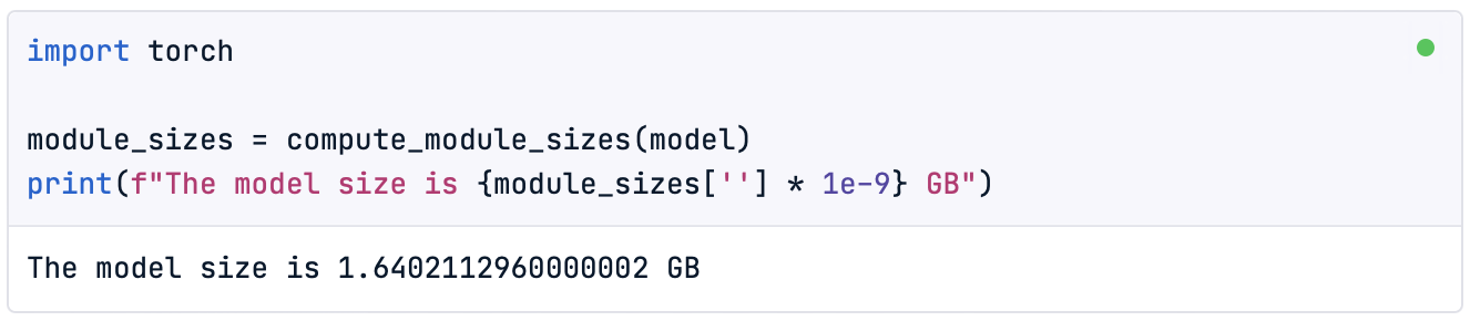

Note: On the DataCamp DataLab we can find the method compute_module_sizes() implemented.

Finally, we can also visualize the dense tensors of the original model as follows:

print(model.gpt_neox.layers[0].attention.dense.weight)

As we can observe, it does resemble the unquantized matrix we have been working with during this article.

2. Quantize. The quantize() method allows the conversion of the default standard float model into a quantized model straightaway.

from quanto import quantize, freeze
quantize(model, weights=torch.int8, activations=None)

In this case, we are quantizing only the weights of the model to an int8 data type. This method converts the model to use lower precision arithmetic including the calibration step.

If we now print the layers of the model, we will see that the original linear layers (Linear) have been replaced with quantized linear layers (QLinear):

print(model)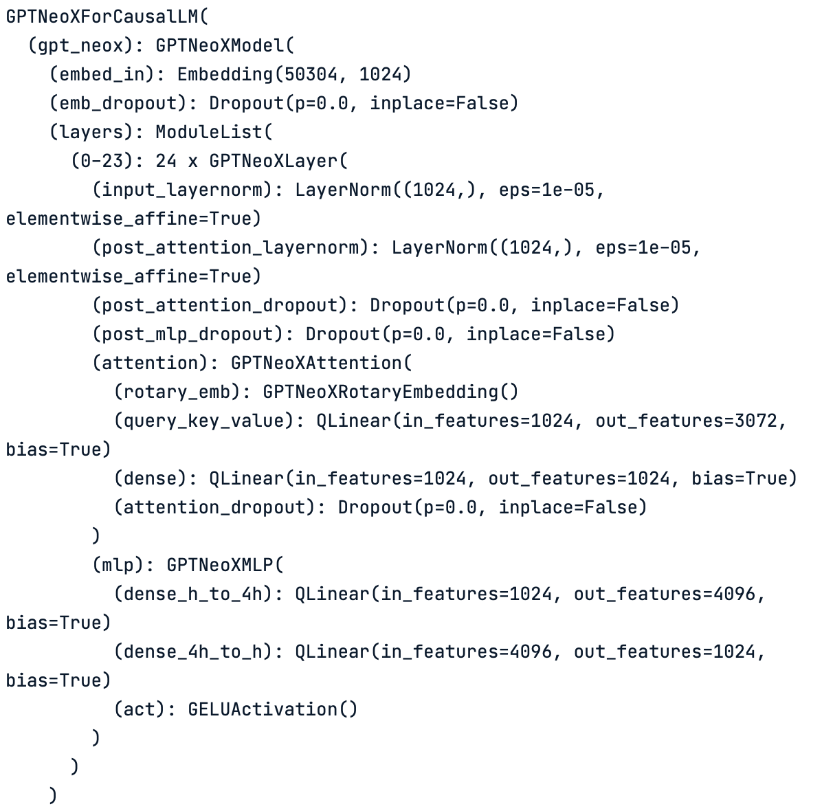

Layer-by-layer schema of the quantized model. Note how all the original linear layers have turn into quantized linear layers (QLinear).

Nevertheless, if we print the matrix of weights, we will see that they have not been transformed:

print(model.gpt_neox.layers[0].attention.dense.weight)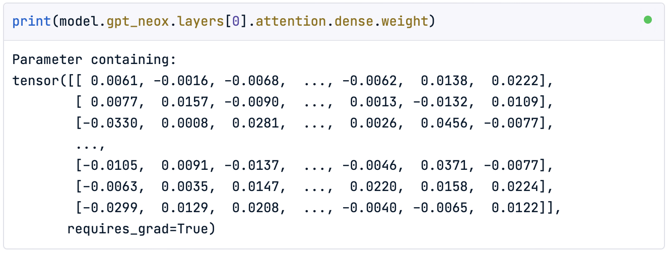

3. Freeze. To apply the quantization effect to the weights, we need to use the freeze() method.

freeze(model)

This method embeds the quantization parameters into the model, effectively converting the weights to the target data type. Let’s observe now the quantized model parameters:

print(model.gpt_neox.layers[0].attention.dense.weight)

As we can see, the weights are now within the range of the Pytorch int8 data type.

4. Final checks. Once the model is quantized, we can check the new reduced model size:

module_sizes = compute_module_sizes(model)
print(f"The model size is {module_sizes[''] * 1e-9} GB")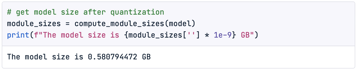

We have achieved a model that is only 35% of the original size!

Finally, let’s check the new performance of the model with a simple inference:

outputs = model.generate(**inputs, max_new_tokens=10)
print(tokenizer.decode(outputs[0], skip_special_tokens=True))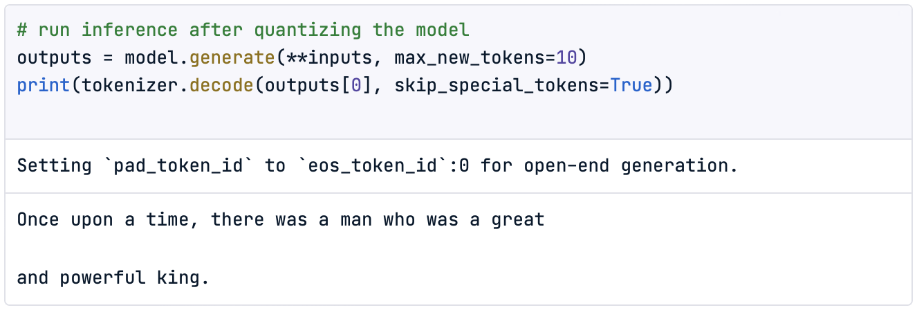

Of course, checking the performance with one single inference is not meaningful, so it would be a good practice to define a quantitative method to evaluate it.

Now it is your time to try!

Conclusion

The increasing memory demands of LLMs limit both their training and hosting for inference, consequently restricting the accessibility and adoption of LLM-based applications. 

In this article, we have introduced the concept of quantization, which involves reducing the precision of the model's weights and activations to decrease its memory footprint and computational requirements. This process helps make models more efficient and accessible, particularly for deployment on resource-constrained devices.

We approached this technique by using some examples, rounding the numerical values of the weights. Then, we moved forward to a simple type of quantization known as downcasting. When downcasting a model, parameters are converted to a more compact data type, like bfloat16, for inference. While this enables the model to perform calculations and activations in this smaller data type, performance typically degrades with the size of the data type, being ineffective with integer types like int8.

To address this, we introduced linear quantization, which maintains performance closer to the original model by converting back to float32 during inference. This enables the use of even smaller data types, such as int8.

We walked through the numerical steps of applying linear quantization and implemented our weight quantization using Hugging Face’s Quanto library. Notably, with the Quanto library, we can quantize any PyTorch model, including those available on Hugging Face. 

For those interested in trying out heavier models like LLaMa 2 or Mistral, consider upgrading your DataCamp space to premium for more computing power.

For larger models, we might require extra resources than can be accessed in the DataCamp Premium Plan.

By mastering quantization techniques, we can unlock the full potential of Large Language Models while requiring fewer resources, making advanced AI more efficient, accessible, and versatile.

I hope this article helps you get hands-on with quantization for LLMs!