Snowflake Arctic Tutorial: Getting Started With Snowflake's LLM

Snowflake Arctic is an innovative development in the field of text embeddings, offering a powerful set of tools designed to simplify the process of adopting AI on enterprise data.

In this tutorial, we’ll provide an overview of Snowflake Arctic, go through the setup process, explore integration techniques, and share best practices and troubleshooting tips. We’ll also showcase real-world use cases, discuss future developments, and provide resources for ongoing support and learning.

If you want to learn more about Snowflake, check out this Introduction to Snowflake course.

What Is Snowflake Arctic?

So, what exactly is Snowflake Arctic? It's a comprehensive suite of tools designed to simplify the integration and deployment of AI within the Snowflake Data Cloud. At its core, Snowflake Arctic offers a collection of embedding models that empower us to efficiently extract valuable insights from our data.

Additionally, it includes a versatile general-purpose Large Language Model (LLM) capable of tackling a wide range of tasks, from generating SQL queries and programming code to following complex instructions.

One of Arctic's standout features is its seamless integration with the Snowflake Data Cloud. This tight coupling allows us to leverage the power of AI directly within our existing data infrastructure, ensuring a secure and streamlined experience.

Importantly, all models within the Snowflake Arctic family are available under an Apache 2.0 license, allowing us to use them for both academic and commercial purposes.

Architecture and performance

Snowflake Arctic has three main components:

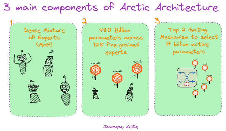
Components of Snowflake Arctic.

Snowflake Arctic's architecture is built upon a Dense Mixture of Experts (MoE) hybrid transformer design, a key innovation that enables efficient scaling and adaptability. This approach leverages a vast network of 480 billion parameters distributed across 128 specialized experts, each fine-tuned for specific tasks.

However, not all experts are activated for every query. Arctic employs a top-2 gating mechanism, selecting only the two most relevant experts for each input, thus activating a mere 17 billion parameters. This optimization significantly reduces computational overhead while maintaining top-tier performance across a wide range of enterprise-focused tasks.

Key features

Snowflake Arctic stands out because of the following four key features:

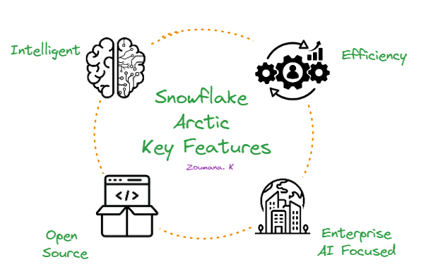
Snowflake Arctic's four key features.

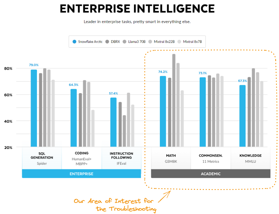
First and foremost, it's remarkably intelligent. Arctic excels at complex tasks like generating SQL queries, writing code, and following detailed instructions. In industry benchmark tests, it consistently outperforms similar models, demonstrating its ability to handle intricate, real-world scenarios.

Second, Arctic is designed for efficiency. Its unique architecture allows it to deliver top-tier performance while consuming fewer computational resources. This translates to significant cost savings, making it an attractive option for organizations of all sizes.

Third, Snowflake Arctic embraces open source. It's available under an Apache 2.0 license, granting everyone access to its code and model weights.

Finally, Arctic is laser-focused on enterprise AI. It's purpose-built to address the specific needs of businesses, delivering high-quality results for tasks like data analysis, process automation, and decision support.

Snowflake Arctic models

To cater to diverse enterprise AI requirements, Snowflake has introduced two primary models within the Snowflake Arctic family:

• Snowflake Arctic Instruct: This variant excels in generating high-quality responses from natural language prompts.
• Snowflake Arctic Base: This version serves as a versatile foundational language model that can be used in various applications without the need for further fine-tuning.

Snowflake Arctic text embedding models

In addition to the main models, Snowflake provides a family of five text embedding models under the Apache 2.0 license—all focused on information retrieval tasks. The table below illustrates the performance of various Snowflake Arctic models on the Massive Text Embedding Benchmark (MTEB) retrieval task, measured by NDCG@10.

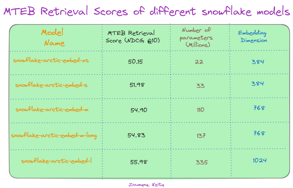
MTEB retrieval scores of different Snowflake models. Source: Hugging Face.

First, we notice there's a general trend of improved performance with increasing model size. The largest model, "snowflake-arctic-embed-l," achieves the highest NDCG@10 score of 55.98, utilizing 335 million parameters and 1024 embedding dimensions. This suggests that model scale plays a significant role in capturing intricate semantic relationships within text data.

Interestingly, increasing the embedding dimension from 384 to 1024 leads to improved scores for the "snowflake-arctic-embed-l" model, highlighting the impact of embedding size on retrieval accuracy. However, a notable exception is the "snowflake-arctic-embed-xs" model. Despite having significantly fewer parameters (22 million), it performs comparably to larger models with the same embedding dimension of 384. This suggests that model efficiency and architectural optimizations can offset the benefits of sheer parameter count in certain scenarios.

Snowflake Arctic: Demo

Before getting our hands dirty on the technical implementation, let’s see the model in action, performing different tasks such as SQL generation, coding, and following instructions.

From the Streamlit demo on Hugging Face, we can provide the model with some requests, adjust the model’s parameters, and get a response.

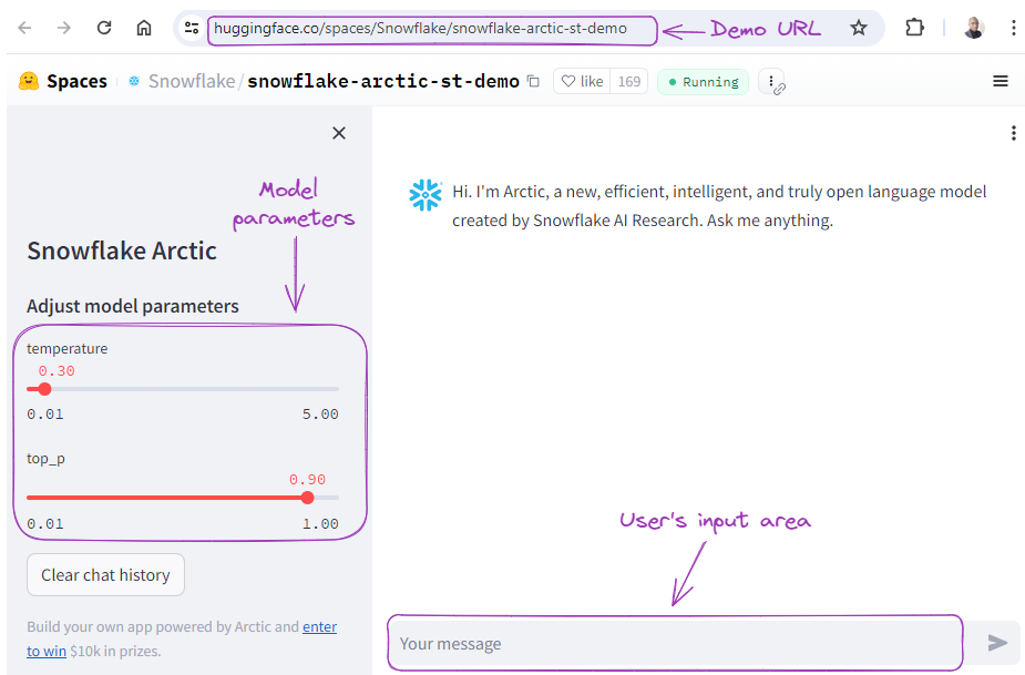
Snowflake Arctic demo.

Let’s first ask the model to generate a SQL query:

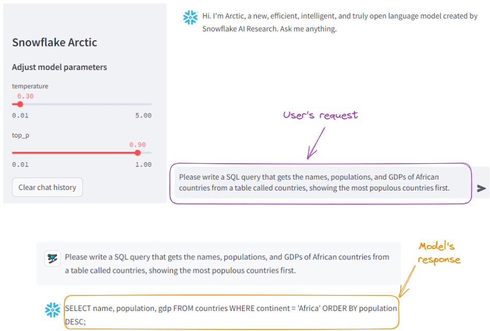
SQL generation example with Snowflake Arctic.

For comparison purposes, let’s submit the same request to ChatGPT-4o: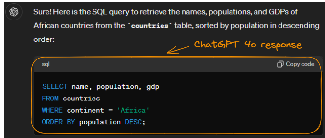

SQL generation example with ChatGPT-4o.

Notice that it generated the same result (with cleaner formatting). We can conclude Arctic did a good job.

Let’s request Arctic to write some Python code:

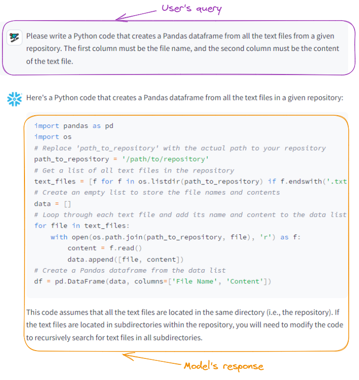
Snowflake Arctic generates Python code.

By providing the same prompt to ChatGPT-4o, we get the following result, which is also accurate:

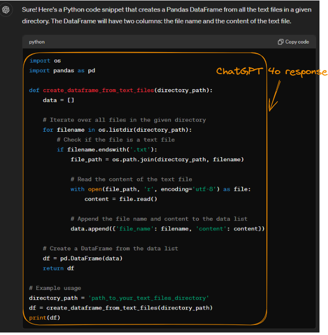
Python code generated by ChatGPT-4o.

While both Arctic and ChatGPT-4o accomplish the same task, their approaches differ in efficiency and memory usage. Both models efficiently read files using os.listdir() and open().

However, ChatGPT-4o's approach of creating a DataFrame from a list of dictionaries might consume slightly more memory than Arctic's method of using a list of lists. This is because Pandas may perform additional processing to handle dictionaries. Despite this minor difference, ChatGPT-4o's modular code structure enhances readability and maintainability.

If you want to learn more about choosing the right LLM, check out this tutorial on LLM Classification: How to Select the Best LLM.

Snowflake Arctic Setup

Now that we know the Snowflake Arctic model's capabilities, let’s focus on accessing and configuring Snowflake Arctic.

Characteristics of the environment

Using Arctic models is resource intensive, so we’ll use the smallest of the Arctic family models, snowflake-arctic-embed-xs, which uses the least computation resources.

Below, we see the characteristics of the environment that we’re using for this tutorial—we display the characteristics by running the nvidia-smi command:

!nvidia-smi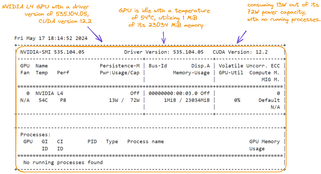

GPU characteristics for the Snowflake Arctic tutorial.

In addition to the NVIDIA L4 GPU, the environment has the following characteristics, which can be found in the Resources section:

• 62.8 GB System RAM
• 22.5 GB GPU RAM
• 201.2 GB Disk

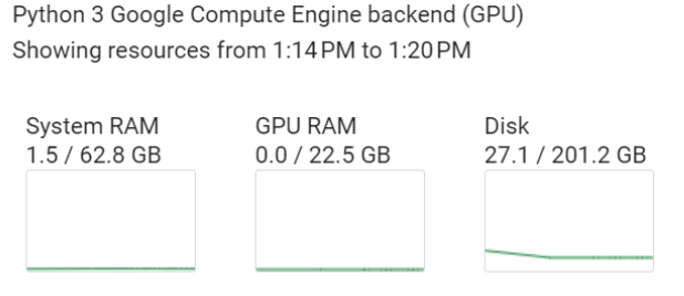
Compute engine backend characteristics.

Installing the libraries

Two main libraries are required for this hands-on tutorial: torch and transformers (we run the code below from a notebook):

%%bash
pip -qqq install transformers>=4.39.0
pip -qqq install torch

We then import the necessary sublibraries:

import torch
from transformers import AutoTokenizer, AutoModel
from torch.nn.functional import cosine_similarity

Load the model and the tokenizer

Let's continue by loading the snowflake-arctic-embed-xs embedding model and its corresponding tokenizer:

model_checkpoint = "Snowflake/snowflake-arctic-embed-xs"
tokenizer = AutoTokenizer.from_pretrained(model_checkpoint)
model = AutoModel.from_pretrained(model_checkpoint, add_pooling_layer=False)

We load the pre-trained model specified by model_checkpoint without an additional pooling layer, which is used to reduce the dimensionality of the model’s output.

Document Similarity Search With Snowflake Arctic

With all the requirements successfully set up, the core use case of this section is to find the top N most similar documents to a given document, along with their cosine similarity scores. To do this, we take these five main steps:

1. Using the embedding model, we generate the embeddings for the initial raw documents.
2. For a given query document, we generate its embedding using the same embedding model.
3. We calculate similarities between query and document embeddings.
4. We return the top N most similar documents along with their similarity scores.

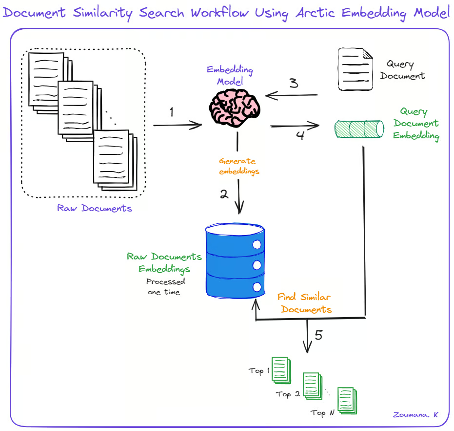
Document similarity search using Snowflake Arctic.

We can implement the steps above using the following helper functions: generate_embedding() and find_similar_documents().

def generate_embedding(document):
    inputs = tokenizer(document, padding=True, truncation=True,
                       return_tensors='pt', max_length=512)
   
    embedding = model(**inputs)[0][:, 0]
    return embedding


def find_similar_documents(query_document, document_embeddings , top_n=5):

    query_embedding = generate_embedding(query_document)
   
    similarity_scores = [cosine_similarity(query_embedding,
                                           doc_embedding).item() for doc_embedding in document_embeddings]

    sorted_indices = torch.argsort(torch.tensor(similarity_scores),
                                   descending=True)

    top_documents = [documents[idx] for idx in sorted_indices[:top_n]]
    top_scores = [similarity_scores[idx] for idx in sorted_indices[:top_n]]

    return top_documents, top_scores

The generate_embedding() function takes a document and input and generates its embedding. The find_similar_documents() takes in a query document, the embeddings of the existing documents, and the desired number of similar documents to be returned.

For simplicity’s sake, we use five simple examples:

documents = [
    "This is a tutorial about Snowflake Arctic Embedding models",
    "Arctic-embed is a state-of-the-art text embedding model.",
    "Snowflake provides various cloud data warehousing solutions.",
    "Embedding models are used for representing text as dense vectors.",
    "The Arctic-embed model is based on the transformer architecture."
]

Next, we generate the embeddings:

document_embeddings = [generate_embedding(doc) for doc in documents]

Let’s pick “What is the Arctic-embed model?” as our query document and find similar documents:

query_document = "What is the Arctic-embed model?"
top_documents, top_scores = find_similar_documents(query_document, document_embeddings)

Finally, we loop across all the top documents to print the document content and its similarity score with the query document.

print("Query Document:")
print(query_document)
print("\nTop Similar Documents:")
for doc, score in zip(top_documents, top_scores):
    print(f"Document: {doc}")
    print(f"Similarity Score: {score:.4f}")
    print()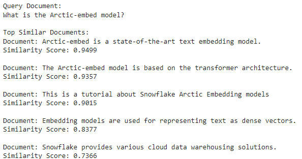

The second document is the most similar because it has the highest cosine similarity score (94.99%).

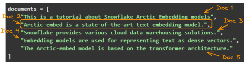
The five original documents.

3D document visualization

When we visualize the documents in a 3D space, we can see the documents that are closer to each other.

The original embeddings have 512 dimensions, which is impossible to visualize. The easiest way is to reduce the dimensions using Principal Component Analysis (PCA). If you want to learn more about PCA, check out this tutorial on Principal Component Analysis (PCA) in Python.

Before using PCA, we need to modify the find_similar_documents() function so that it returns the document embeddings that the PCA will use.

def find_similar_documents(query_document, documents, top_n=5):
    query_embedding = generate_embedding(query_document)
    document_embeddings = [generate_embedding(doc) for doc in documents]

    similarity_scores = [cosine_similarity(query_embedding, doc_embedding).item() for doc_embedding in document_embeddings]
    sorted_indices = torch.argsort(torch.tensor(similarity_scores), descending=True)

    top_documents = [documents[idx] for idx in sorted_indices[:top_n]]
    top_scores = [similarity_scores[idx] for idx in sorted_indices[:top_n]]

    return top_documents, top_scores, document_embeddings

We also import a few modules that are necessary to generate the visualization.

from sklearn.decomposition import PCA
import matplotlib.pyplot as plt
from mpl_toolkits.mplot3d import Axes3D

Now let’s create the 3D visualization by:

• Reshaping the embeddings to fit the PCA input format.
• Reducing the embeddings to three dimensions.
• Creating a 3D visualization of the reduced embeddings.

top_documents, top_scores, document_embeddings = find_similar_documents(query_document, documents)

# Reshape the embeddings
reshaped_embeddings = torch.stack(document_embeddings).detach().numpy()
reshaped_embeddings = reshaped_embeddings.reshape(reshaped_embeddings.shape[0], -1)

# Apply PCA to reduce the embeddings to 3 dimensions
pca = PCA(n_components=3)
reduced_embeddings = pca.fit_transform(reshaped_embeddings)

# Create a 3D plot
fig = plt.figure(figsize=(8, 6))
ax = fig.add_subplot(111, projection='3d')

# Plot the document embeddings
for i, doc in enumerate(documents):
    ax.scatter(reduced_embeddings[i, 0], reduced_embeddings[i, 1], reduced_embeddings[i, 2], marker='o', label=f"Document {i+1}")

# Plot the query document embedding
query_embedding = generate_embedding(query_document)
reshaped_query_embedding = query_embedding.detach().numpy().reshape(1, -1)
reduced_query_embedding = pca.transform(reshaped_query_embedding)
ax.scatter(reduced_query_embedding[0, 0], reduced_query_embedding[0, 1],
           reduced_query_embedding[0, 2], marker='*', s=100, color='red',
           label="Query Document")

ax.set_xlabel('PC1')
ax.set_ylabel('PC2')
ax.set_zlabel('PC3')
ax.legend()
plt.title('Document Embeddings in 3D Space')
plt.show()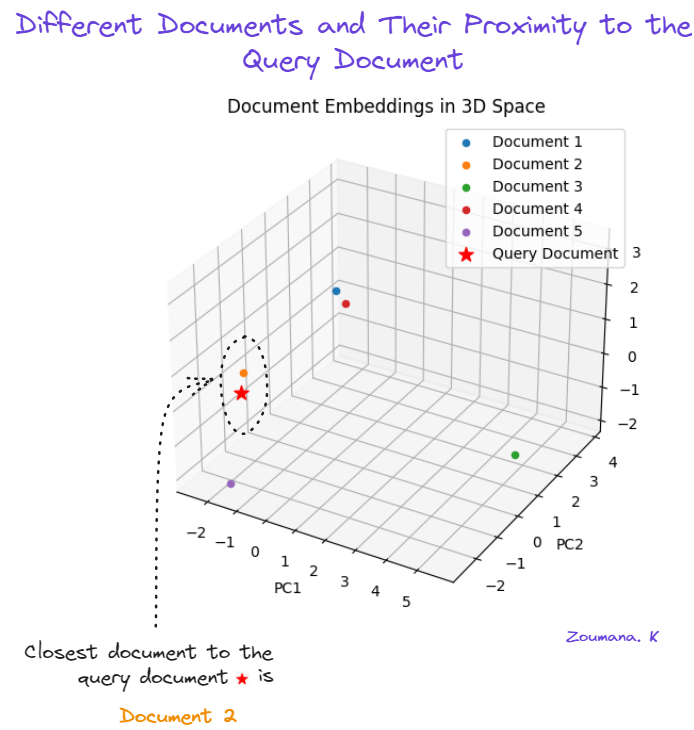

Using PCA to visualize document similarity.

The second document (orange) is the closest to the query document (red star). The fifth document (purple) is the second closest document, while the third document (green) is the furthest.

Integrating Snowflake Arctic With Streamlit

Notebooks are powerful tools for experimentation and rapid visualization, making them popular among data scientists and researchers. However, notebooks may not be the most suitable choice when it comes to deploying models or applications in production environments. This is where Streamlit comes into play.

Streamlit is a Python library that facilitates the development of interactive web applications for data science and machine learning projects. It makes it easy to transform data science projects into production-ready applications without extensive web development knowledge.

Below is the landing page of what we’ll build in this section.

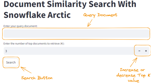
The landing page of the Streamlit application.

Teaching Streamlit is outside the scope of this tutorial, but you can learn it from scratch in this Python Tutorial: Streamlit.

Basic integration techniques

In this section, we’ll explore how to use Streamlit to create a web application for our document similarity search project. To run a Streamlit application, the code needs to be in a Python file (with a .py extension) and execute the following command in the terminal:

streamlit run app.py

However, the first step to using Streamlit is installing it with the pip command:

pip install streamlit

The code we used to build the Streamlit application is a bit long so take your time to go over it. We’ll also explain it after the code block.

import streamlit as st
from transformers import AutoTokenizer, AutoModel
import torch
from torch.nn.functional import cosine_similarity
from sklearn.decomposition import PCA
import matplotlib.pyplot as plt
from mpl_toolkits.mplot3d import Axes3D


model_checkpoint = "Snowflake/snowflake-arctic-embed-xs"
tokenizer = AutoTokenizer.from_pretrained(model_checkpoint)
model = AutoModel.from_pretrained(model_checkpoint, add_pooling_layer=False)


def generate_embedding(document):
    inputs = tokenizer(document, padding=True, truncation=True, return_tensors='pt', max_length=512)
    embedding = model(**inputs)[0][:, 0]
    return embedding


def find_similar_documents(query_document, documents, top_n=5):
    query_embedding = generate_embedding(query_document)
    document_embeddings = [generate_embedding(doc) for doc in documents]


    similarity_scores = [cosine_similarity(query_embedding, doc_embedding).item() for doc_embedding in document_embeddings]
    sorted_indices = torch.argsort(torch.tensor(similarity_scores), descending=True)


    top_documents = [documents[idx] for idx in sorted_indices[:top_n]]
    top_scores = [similarity_scores[idx] for idx in sorted_indices[:top_n]]


    return top_documents, top_scores, document_embeddings


# Sample documents
documents = [
    "This is a tutorial about Snowflake Arctic Embedding models",
    "Arctic-embed is a state-of-the-art text embedding model.",
    "Snowflake provides various cloud data warehousing solutions.",
    "Embedding models are used for representing text as dense vectors.",
    "The Arctic-embed model is based on the transformer architecture."
]


# Streamlit app
st.title("Document Similarity Search With Snowflake Arctic")


query_document = st.text_input("Enter your query document:")
top_k = st.number_input("Enter the number of top documents to retrieve (K):", min_value=1, value=3, step=1)


if st.button("Search"):
    top_documents, top_scores, document_embeddings = find_similar_documents(query_document, documents, top_n=top_k)


    st.subheader("Top {} Similar Documents:".format(top_k))
    for i, (doc, score) in enumerate(zip(top_documents, top_scores)):
        st.write("{}. Document: {}".format(i+1, doc))
        st.write("   Similarity Score: {:.4f}".format(score))


    # Reshape the embeddings
    reshaped_embeddings = torch.stack(document_embeddings).detach().numpy()
    reshaped_embeddings = reshaped_embeddings.reshape(reshaped_embeddings.shape[0], -1)


    # Apply PCA to reduce the embeddings to 3 dimensions
    pca = PCA(n_components=3)
    reduced_embeddings = pca.fit_transform(reshaped_embeddings)


    # Create a 3D plot
    fig = plt.figure(figsize=(8, 6))
    ax = fig.add_subplot(111, projection='3d')


    # Plot the document embeddings
    for i, doc in enumerate(documents):
        ax.scatter(reduced_embeddings[i, 0], reduced_embeddings[i, 1], reduced_embeddings[i, 2], marker='o', label=f"Document {i+1}")


    # Plot the query document embedding
    query_embedding = generate_embedding(query_document)
    reshaped_query_embedding = query_embedding.detach().numpy().reshape(1, -1)
    reduced_query_embedding = pca.transform(reshaped_query_embedding)
    ax.scatter(reduced_query_embedding[0, 0], reduced_query_embedding[0, 1], reduced_query_embedding[0, 2], marker='*', s=100, color='red', label="Query Document")


    ax.set_xlabel('PC1')
    ax.set_ylabel('PC2')
    ax.set_zlabel('PC3')
    ax.legend()
    plt.title('Document Embeddings in 3D Space')


    st.pyplot(fig)

Using the code above, we created a Streamlit app named "Document Similarity Search With Snowflake Arctic." Let’s make a few observations about the code:

• It allows the user to enter a query document using st.text_input() and specify the number of top documents to retrieve (K) using st.number_input().
• When the user clicks the Search button (st.button("Search")), the find_similar_documents() function is called with the query document, the list of documents, and the specified top_k value.
• The app displays the top K similar documents along with their similarity scores using st.subheader() and st.write().
• The document embeddings are reshaped and reduced to 3 dimensions using PCA for visualization purposes.
• A 3D plot is created using Matplotlib to visualize the document embeddings and the query document embedding.
• The 3D plot is displayed in the Streamlit app using st.pyplot(fig).

The Streamlit section of the code focuses on creating an interactive user interface where users can input a query document, specify the number of top similar documents to retrieve, and view the results along with a 3D visualization of the document embeddings.

The complete code of the article is available in this Jupyter Notebook.

We can start the application with the streamlit run app.py command, which will get us to the landing page. By providing the same query document and setting Top K to 3, we get the following result:

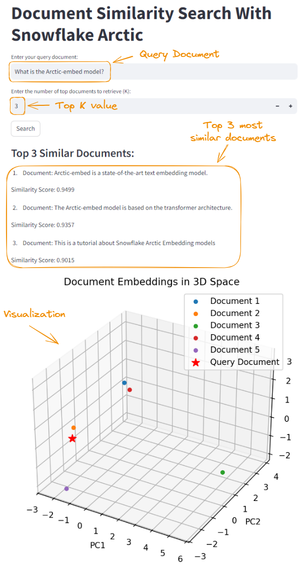
Snowflake Arctic integration using Streamlit.

Advanced configuration tips

When working with large language models like Arctic, it's crucial to thoroughly test and validate configurations within our target environment. This ensures optimal performance and reliability. Here are some configuration tips to keep in mind:

• Quantization: Lower the precision of weights to reduce model size and speed up inference. At the time of writing this article, the quantized checkpoint is not available and should be available in the future for both Hugging Face inference and vLLM.
• Hardware acceleration: Utilize GPUs and mixed-precision training and inference.
• Model distillation: Train a smaller "student" model to mimic a larger "teacher" model.
• Caching and preprocessing: Store frequently used embeddings and preprocess data offline.
• Monitoring and logging: Track performance, resource usage, and errors for optimization.
• Scaling and load balancing: Deploy multiple instances and distribute requests evenly.
• Security and access control: Implement authentication, authorization, and secure communication.
• Continuous optimization: Monitor, analyze, and experiment with new techniques regularly.

Best Practices and Troubleshooting

To ensure optimal performance and smooth operation of Snowflake Arctic, it's crucial to follow best practices and be prepared to troubleshoot any possible issues. In this section, we'll explore tips and tricks for enhancing performance based on real-world benchmarks and academic research.

Source: Arctic Cloud.

Here are some tips and tricks to enhance its capabilities:

• Utilize vectorized execution engine for faster math computations (GSMBK).
• Cache frequently accessed academic datasets and pre-computed results.
• Optimize data loading with bulk techniques and local staging.
• Minimize data movement by computing closer to storage.
• Leverage parallel processing for computationally intensive tasks (GSM8K, MMLU).
• Monitor performance on academic benchmarks and resolve bottlenecks.
• Collaborate with the academic community and incorporate the latest research findings.
• Continuously test and benchmark performance to identify areas for improvement.

Inference performance

Snowflake Arctic's performance stands out in both inference and training scenarios. During inference, it consistently delivers a superior performance/cost ratio compared to other models. This efficiency improves as more parameters are activated, maintaining a significant advantage even at around 60 billion active parameters, outperforming competitors like Mixral and Llama 3.

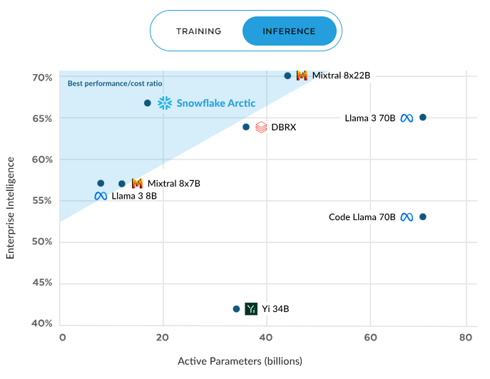
Arctic inference efficiency. Source: Snowflake.com.

Training performance

The trend continues in training, where Arctic again boasts the best performance/cost ratio. This efficiency scales with increased compute, reaching approximately 70% at 16X compute, far exceeding models like DBRX, Llama 3, Code Llama, and Yi. These results underscore Arctic's value proposition: high-quality performance at a fraction of the computational cost, making it a compelling choice for resource-conscious enterprises.

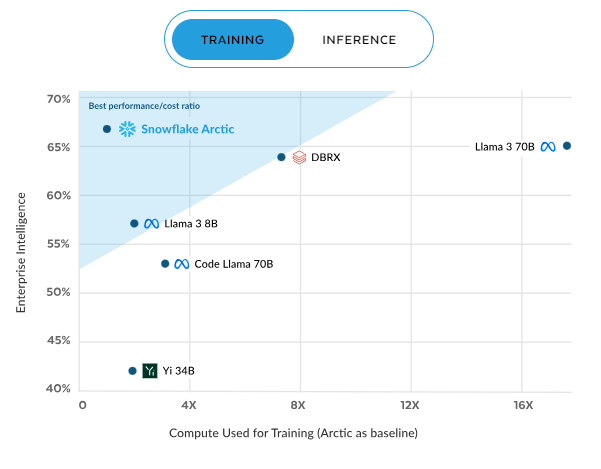
Arctic training efficiency. Source: Snowflake.com.

Some tips and tricks for optimizing the performance for inference and training include, but are not limited to:

• Leverage Snowflake's scalable architecture for training Snowflake Arctic on large datasets.
• Use Snowflake's distributed computing to parallelize training workloads and reduce time.
• Use Snowflake's data caching to store frequently accessed data and intermediate results, speeding up training.
• Optimize data loading with bulk loading techniques and local staging to maintain performance and reduce costs.
• Monitor training progress and performance metrics with Snowflake's tools and custom solutions.
• Perform hyperparameter tuning to balance model performance and training costs.
• Use Snowflake's cost-efficient compute resources for scalable inference workloads.
• Implement efficient inference pipelines using Snowflake's data warehousing capabilities.
• Continuously monitor and analyze inference performance metrics for optimization opportunities.

The Future of Snowflake Arctic

Snowflake Arctic's impressive performance and cost-efficiency have set a new standard for language models. Future development may include advanced natural language understanding, improved multi-task learning, and better support for domain-specific applications. As Snowflake innovates, users can expect even more powerful and versatile tools.

Snowflake offers a great community and comprehensive support resources. Users can connect, share knowledge, and learn from each other on the Snowflake community forums. Detailed documentation and tutorials are available on the official website to help users navigate and maximize Snowflake Arctic's features.

Conclusion

Snowflake Arctic is a game-changer in the field of text embeddings, offering a powerful and efficient solution for enterprises seeking to unlock the full potential of their data. Its seamless integration with the Snowflake Data Cloud and scalable architecture makes it an ideal choice for organizations looking to streamline their data retrieval and analysis processes.

Throughout this guide, we’ve explored Snowflake Arctic's core capabilities, covering everything from its setup and configuration to advanced integration techniques and practical applications. By leveraging its advanced features and performance optimizations, enterprises can achieve better efficiency and accuracy in their text embedding operations.

If you want to learn more about Snowflake, check out this Snowflake Tutorial for Beginners.