How to Multiply in Excel: Multiply Cells, Columns, Rows, and More

In this guide, I’ll show you different ways to multiply numbers in Excel. We’ll start with the basics using the * symbol to multiply numbers, then move on to multiplying entire columns and rows, and even using built-in functions like PRODUCT() and SUMPRODUCT(). By the end, you’ll understand how to multiply efficiently in Excel, regardless of the data you’re working with.

However, if you’re new to Excel, check out our Introduction to Excel course to understand the basics first.

The Quick Answer: How to Multiply in Excel

To multiply, type an equals sign = and numbers separated by an asterisk *.

For example, if I want to multiply 4 by 5, my expression will look this: 

=4*5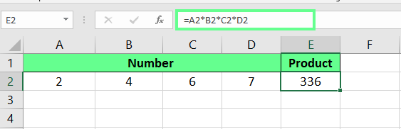

How to multiply in Excel. Image by Author.

How to Multiply Cells in Excel

Apart from basic numbers, we can even multiply cells for quicker calculations. Whether it's two cells or more, the process stays the same — the only difference is we use cell references instead of fixed numbers here. 

How to multiply two cells in Excel

Let's say cells A2 and B2 contain numbers. In cell C2, I enter =A2*B2 and press Enter. If I change the value in any of the first two cells, it will automatically update the result.

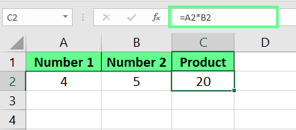
Multiply two cells. Image by Author.

How to multiply multiple cells in Excel

If we want to multiply more than two cells, we can extend the formula like this:

=A2*B2*C2*D2

Multiply multiple cells. Image by Author.

How to Multiply Columns and Rows in Excel

We can also multiply entire columns and rows in Excel. Let’s see how:

How to multiply columns in Excel

If I want to multiply multiple columns. I’ll enter the following formula in the cell D2: 

=A2*B2*C2

Once I hit Enter, the result will be calculated. Now, instead of repeating the formula to the other cells, I can drag or double-click on the small green square at the corner of the cell to copy down the formula to the last cell.

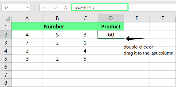
Multiply two columns. Image by Author.

If any cell is empty but referenced in a formula, Excel treats it as 0. So the formula will return 0.

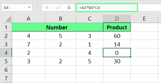
Multiply multiple columns. Image by Author.

How to multiply columns by a number in Excel

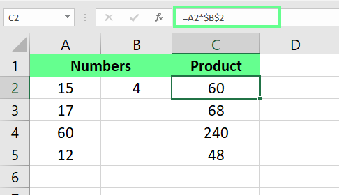
If I want to multiply the whole column by a single number, I will use the absolute reference $. This means the entire column from A2 to A5 is multiplied by a number in cell B2. My formula will look like this: 

=A2*$B$2

Here, the symbol $ will fix the value of B2, which tells Excel to use that value on every cell when I drag the formula down the column. 

Note: We don’t have to type $ manually. Click on the cell name in the formula, like in my case, B2, and press the F4 key. This will automatically fix the formula.

Multiply columns with an absolute reference. Image by Author.

How to multiply rows in Excel

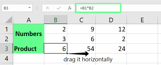
Rows work the same way as columns but run horizontally instead of vertically. If I want to multiply row 1 (B1) by row 2 (B2), I will enter

=B1*B2

in a new cell and drag it horizontally to copy it to the rest of the row.

Multiply multiple rows. Image by Author.

How to multiply rows by a number in Excel

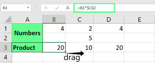
I can use an absolute reference to multiply an entire row by a single number. For example, if the multiplier is in cell C2 and the values are in row 1, I type

=B1*$C$2

in another cell. Then, I drag the formula across the row to apply the multiplication to the whole row.

Multiply rows with an absolute reference. Image by Author.

How to Multiply Using Functions in Excel

Excel also has some built-in functions to find the product of numbers. Let’s see what are some commonly used ones and how they work:

Using Excel's PRODUCT() function

We can use the PRODUCT() function in Excel to multiply multiple numbers and ranges all at once. The syntax is simple: 

=PRODUCT(number1, [number2], ...)

Here number1, number2, and so on, are the ranges or numbers we want to multiply. 

If I want to multiply all the values in cells A2 to A5. I use the formula:

=PRODUCT(A2:A5)

And if I want to multiply the result with any number like 5, my formula will look like this:

=PRODUCT(A2:A5, 5)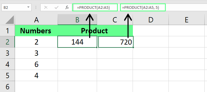

Multiply cells using the PRODUCT() function. Image by Author.

This is helpful when we work with large datasets or want a clean and compact formula instead of writing it manually. What I also like about this formula is that if a cell is empty but referenced in the formula, it will not return 0. This way, I can reference cells where data will be added later, and the formula will still work perfectly.

Using Excel's SUMPRODUCT() function

The SUMPRODUCT() function multiplies two or more lists of numbers and then sums up the results. Its syntax is: 

=SUMPRODUCT(array1, [array2], [array3], ...)

If I want to calculate the total sales of items by multiplying the quantity sold by the price for each item, I can use this formula:

=SUMPRODUCT(B2:B6, C2:C6)

If I were to calculate it manually, the calculation would look like this: (B2*C2)+(B3*C3)+(B4*C4)+(B5*C5). But with SUMPRODUCT(), Excel does all the work in one step, which makes the process more efficient.

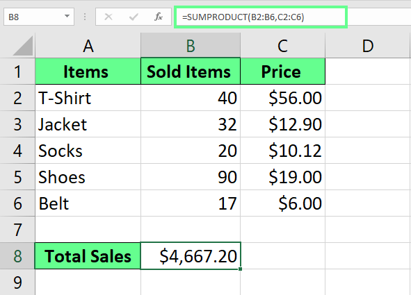
Multiply and sum using the SUMPRODUCT() function. Image by Author.

This function also works perfectly for financial modeling and data analysis, as we often have to calculate weighted totals and analyze relationships between datasets in these fields.

Other Things That Might Come Up

Finally, let's take a look at a couple of other interesting things that might come up.

Multiplying by percentages in Excel

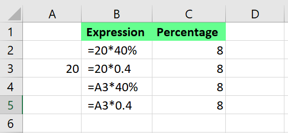
We can even multiply by percentages in Excel to calculate portions or adjustments. There are two ways to do this: multiply with percentages directly or use decimal equivalents. Let’s understand each:

Direct multiplication with percentages

If I want to multiply a number by a percentage in Excel, I just type = followed by the number, then *, and the percentage with a % sign. For example, to find 40% of 20, I enter

=20*40%

in a cell, which gives 8.

The % sign automatically converts the number into a percentage, which makes calculations easier for me. 

Using decimals instead of percentages

We can also use decimals instead of percentages. For example, I know 40% means 0.4 in decimals, so I can write this formula to find the result, which is 8:

=20*0.4

I can also replace the hardcoded number with the cell reference. (We have 20 in A3, so I referenced it in the formula and see how it gives an accurate answer.)

Multiply a cell and number by a percentage. Image by Author.

Matrix multiplication in Excel using array formulas

Now, it may sound complicated, but we can even multiply matrices in Excel. Luckily, Excel makes the process as simple as possible with the MMULT() function. 

MMULT() works by multiplying two matrices. It takes each row from the first matrix, multiplies it by each column from the second matrix, and then adds the results. Its syntax is: 

=MMULT(array1, array2)

The resulting matrix will have the same number of rows as the first matrix and the same number of columns as the second matrix.

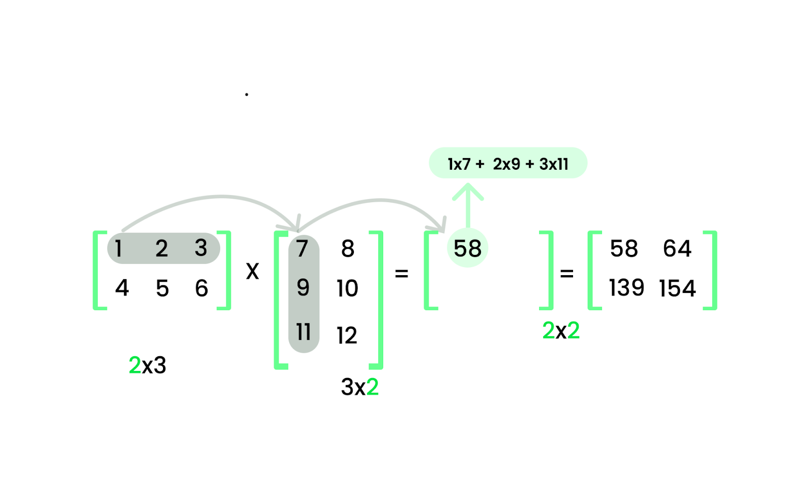
Matrix multiplication. Image by Author.

For example, I have a 2×3 matrix and a 3×2 matrix. The result will be a 2×2 matrix. So, I first select a 2×2 range where I want the result to appear. Then, I type the following:

=MMULT(B2:D3, C5:D7)

Finally, I press Ctrl + Shift + Enter to apply the formula.

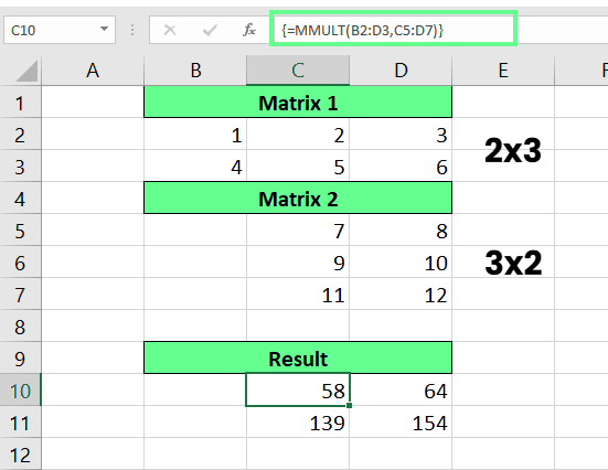
Multiply matrices using the MMULT() function. Image by Author.

When I use MMULT(), I always check for two things: 

1. The number of columns in the first matrix must match the number of rows in the second matrix — otherwise, the function won’t work. 

2. All the cells must have numbers only because if there are empty cells or text, Excel will give a #VALUE! error.

If you are serious about becoming better at linear algebra specifically, try our Linear Algebra for Data Science in R course, which will operations like matrix multiplication.