How to Use Jupyter Notebooks: The Ultimate Guide

Jupyter notebooks are documents for technical and data science content. This tutorial provides an overview of Jupyter notebooks, their components, and how to use them. 

We will explore notebooks using DataLab, a hosted notebook service that provides all the functionality of Jupyter notebooks, along with functionality for connecting to databases, real-time collaboration, and publishing your work. 

This tutorial assumes that you have used a data science programming language before, such as Python, SQL, R, or Julia.

Overview of notebooks

Notebooks combine computer code (such as Python, SQL, or R), the output from running the code, and rich text elements (formatting, tables, figures, equations, links, etc.) in a single document. 

The key benefit of notebooks is the ability to include commentary with your code. That means that you can avoid the error-prone process of copying and pasting analysis results into a separate report. Instead, you simply mix your analysis with the report text in the notebook.

Who should use Jupyter Notebooks?

Jupyter Notebooks are primarily used by data professionals, particularly data analysts and data scientists. According to the Kaggle Survey 2022 results, Jupyter Notebooks are the most popular data science IDE, used by over 80% of respondents. 

Types of Jupyter Notebook

There are two main types of Jupyter Notebook; hosted and local notebooks. DataCamp provides DataLab, a hosted Jupyter Notebook that we will use for the majority of this tutorial. DataLab is an excellent option for learners and professionals who do not want to set up a local environment. 

Except where noted, the functionality described in this tutorial will work on other Jupyter notebook versions. If you prefer to use a local environment, you can install Jupyter Notebook on your machine using our Installing Jupyter Notebook tutorial. Marcus Schanta maintains a list of other hosted notebook platforms.

Components of a notebook

A Jupyter Notebook consists of three main components: cells, a runtime environment, and a file system.

 Cells are the individual units of the notebook, and they can contain either text or code:

• Text cells are used to write narrative text and include images, links, and equations.
  • Text cells are written in Markdown, a simple markup language.
• Code cells are used to write and execute code. 
  • The output from code cells will be displayed directly below the code cell. 
• SQL cells (DataLab only) are used to execute SQL queries, which means you can easily retrieve data from a database.
• Chart cells (DataLab only) can be used to create visualizations and quickly visualize Pandas dataframes.

The runtime environment is responsible for executing the code in the notebook. The runtime environment can be configured to support different languages, including Python, R or SQL.

The filesystem allows you to upload, store, and download data files, code files, and outputs from your analysis.

Command mode and edit mode

Jupyter notebooks have two different modes of interaction: command mode and edit mode. In command mode, you can navigate between cells, add and delete cells, and change the cell type. In edit mode, you can edit the contents of a cell.

In order to enter command mode, you can either press Escape or click outside a cell. To enter edit mode, you can press Enter or click inside a cell.

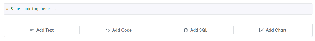
In DataLab, you can click the ‘Add Text’ or ‘Add Code’ buttons to add a new cell.

Getting help

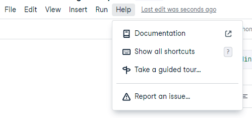
For Jupyter notebook, you can get help using the documentation or using the option in the menu. In DataLab, help and keyboard shortcuts can be quickly accessed by pressing the help button in the menu.

Writing text

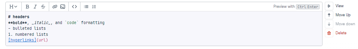
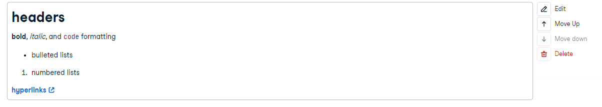
Text cells are written in the Markdown markup language, allowing you to easily write and format text. While in edit mode, you can use syntax such as ** ** for bold, or use the buttons, to format your text. 

Here are a few different options:

Pressing shift + enter or the ‘View’ button will run the cell, giving the following result.

• Lines beginning # are a top-level header. Start with ## for a second-level header, ### for a third-level header, and so on.
• Surround text in ** to make it bold, __ to make it italic, and ` to make it code formatted.
• Start consecutive lines with - to make them into a bulleted list.
• Start lines with numbers followed by a period to make them into a numbered list.
• Hyperlinks are written in two parts. The text to display is surrounded by square brackets, then the url is surrounded by parentheses.

Writing and running code

Pressing ‘Add Code’ or entering a command with (escape) and pressing ‘B’ will add a new code block.

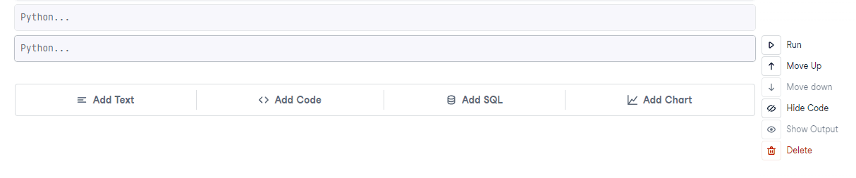
Write code in the cell just as you would in a script.

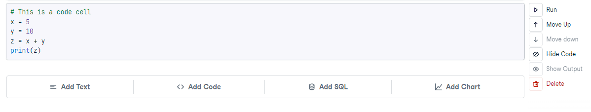
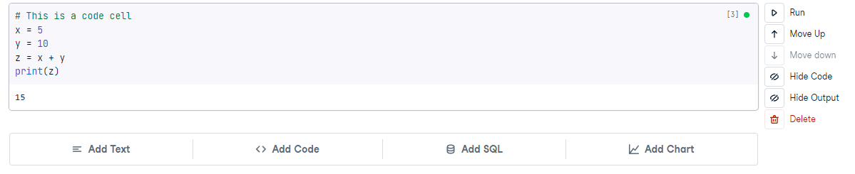
Pressing Run or CTRL/CMD+Enter runs the code and displays its output.

Reading and writing files

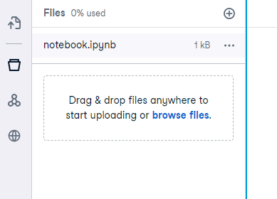
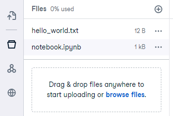
Pressing ‘Browse and upload files’ on the left-hand menu brings up the file system, and pressing the ‘plus’ will allow you to upload a file from your local machine. Below, we have uploaded a simple text file called hello_world.txt.

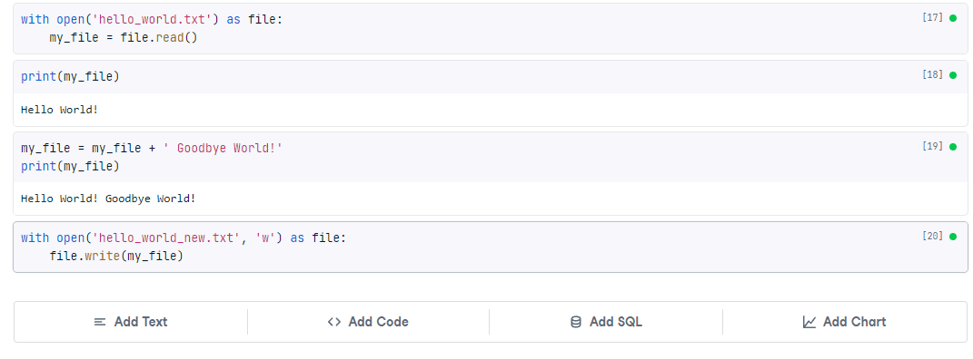
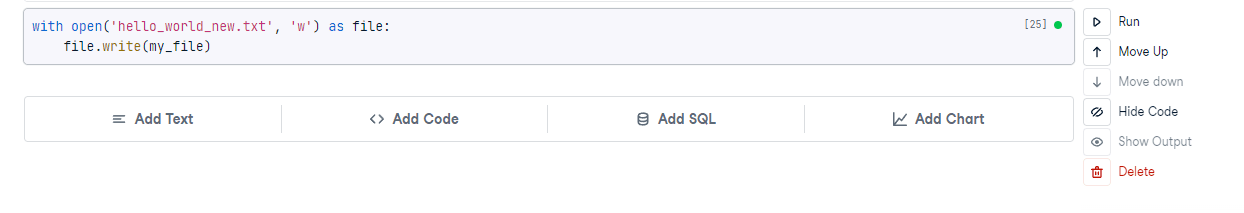
We can use the following code to open the file, add some text, then save a new file.

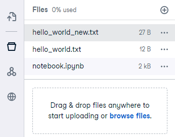
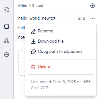
You’ll now see the new file in the file system, and it will contain our updates.

Working with the File System

We have shown how to upload, update and create a new file. To download the new file, press the three dots in the file system and hit download.

The plus button used to create new files can also be used to create fresh notebooks, which will have no cells or output. 

Commanding cells

You can quickly reorder cells with the move up and move down buttons, as shown in the image below. 

This will reorder your code. (Note that your code may break if you try and run it in the wrong order!)

The Hide Code button will collapse and hide the code; this is useful for very long code blocks that you aren’t currently working on. It is also useful if the readers of your analysis don't care about the technical details and only want to see the results.

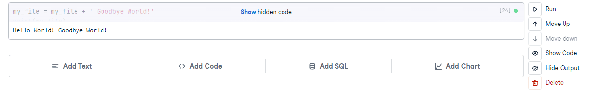
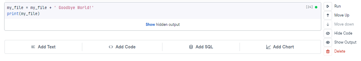
Similarly, the Hide Output button allows you to hide long outputs. 

These buttons can also be used together to hide both code and output.

Publishing reports (DataLab only)

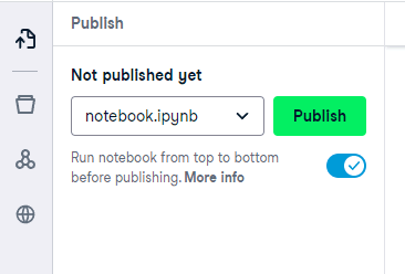
DataLab allows you to publish your notebooks as publications. This is a great way to showcase your excellent work and collaborate with other data scientists.

You can publish your notebook by pressing the ‘Publish’ button on the side menu. From there, hit publish to share your notebook. It is a good idea to run the notebook from top to bottom before publishing. This helps to check your code and ensures it is readable, as most people will read from top to bottom.

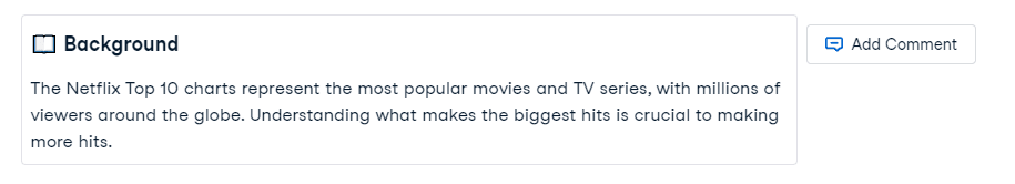
Once your notebook has been published, other users can view the publication and comment on individual cells. You can also do the same to others. This is a great way to open up discussion or understand a complex piece of code. Here’s a Workplace example: 

Sharing Jupyter Notebooks (DataLab only)

Sharing workbooks is another useful DataLab-only function. Because the notebook is hosted, you can share a public or private, access-controlled link that the receiver can run themselves. 

This is a fantastic way to collaborate. Data Science is a deep and wide field, meaning no single person is expected to know everything. Data scientists must collaborate to get the best results, whether it’s efficient code, compelling visualizations, or an accurate model. DataLab allows real-time collaboration, where multiple people can edit a notebook at once.

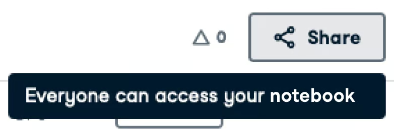
To share your notebook, press the share button on the top right. Here you can copy the link, make the notebook private/public, and set who can access the notebook (if private).

Take it to the next level

Start your data science journey today by signing up for DataLab for free. If you get stuck, the DataLab Documentation is a great place for more information.