FIFA World Cup 2026 Winner Prediction: An MLOps Guide

The Data Behind the Predictions

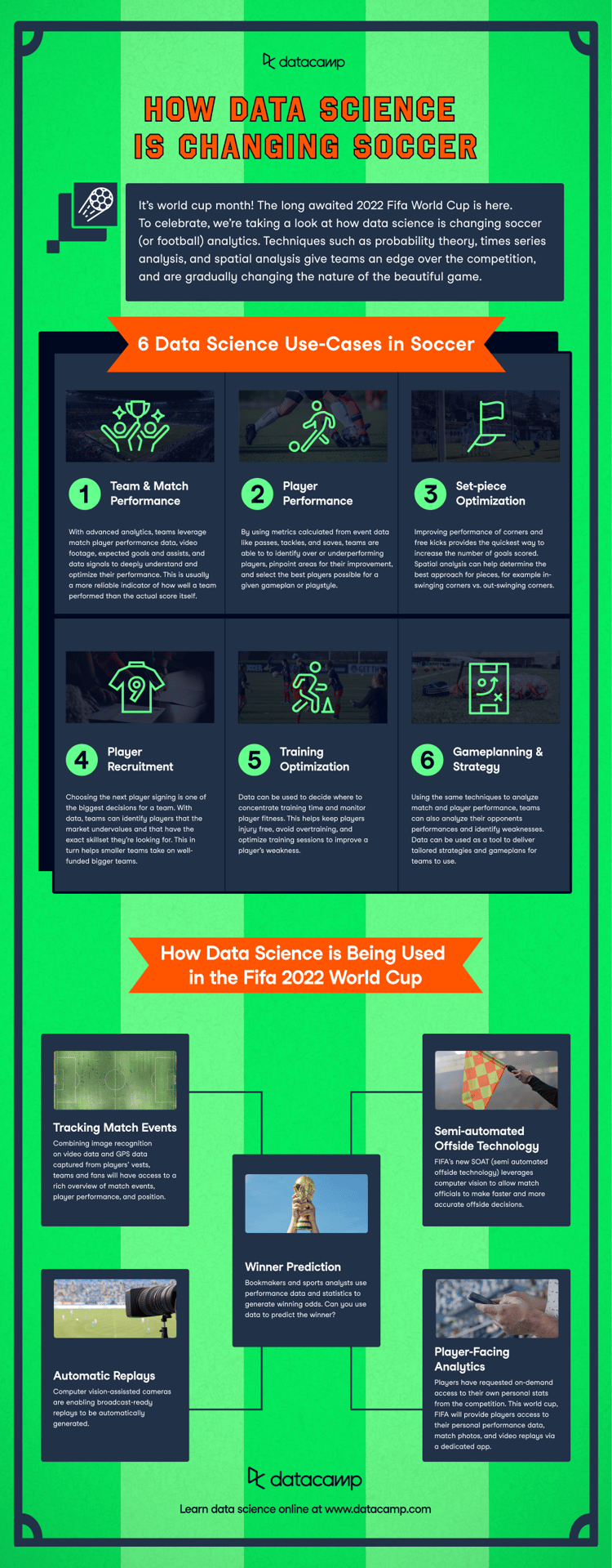
A prediction is only ever as good as what goes into it, so it is worth starting with the raw materials. The model learns from two live data sources and turns them into a single, tidy table of features.

Where the data comes from

Everything is built from two places. API-Football supplies the fixtures and per-match statistics: who played whom, when, where, and how it ended. eloratings.net supplies Elo ratings for every national team.

An Elo rating is a single number that captures how strong a team is. Every team sits somewhere on the scale, and after each match, the rating updates: beat a stronger side, and you gain a lot; lose to a weaker one, and you drop sharply. The idea comes from chess and adapts neatly to football. If you want the full intuition, this earlier DataCamp piece walks through it in the context of the 2022 World Cup.

Together, the two sources give a Gold dataset of roughly 6,900 international matches since 2018 to learn from.

What the model predicts

Here is the first important design choice. Instead of predicting the outcome directly as a win, draw, or loss, the model predicts something more granular: the number of goals each team scores in a match. Goal counts in football follow, to a good approximation, a Poisson distribution, the standard way to model how often a relatively rare event happens in a fixed window of time.

Predicting goals rather than results is what makes everything later possible. Once the model can produce a plausible scoreline for any matchup, the questions everyone actually cares about, who escapes the group and who lifts the trophy, can be answered by simulating those scorelines thousands of times.

The features that matter

Each match is described by a small, carefully chosen set of features:

• Elo difference: the gap in rating between the two teams. This is by far the single most important feature in the model, with an importance roughly two orders of magnitude above the next strongest. That fits intuition, as the strength gap between the two sides tells you more about the likely result than almost anything else.
• Elo sum: the two ratings added together, a stand-in for the overall quality of the fixture. The difference alone cannot tell Argentina against Spain apart from San Marino against Andorra, two evenly matched games at completely different levels, and the sum restores that information.
• Rolling Elo change (last 5 matches): how much each team's rating has shifted recently. This captures form while already accounting for the strength of the opponents faced.
• Rolling goals for and against (last 5 matches): recent attacking and defensive output in absolute terms, calculated for each team.
• Match context: the competition tier (a World Cup game carries different weight from a qualifier or a Nations League fixture), whether the match is a knockout, and whether it is played at a neutral venue.

Every feature is strictly leakage-safe, meaning each one uses only information that was available before kickoff. That sounds obvious, but it is one of the easiest ways to accidentally build a model that looks brilliant in testing and falls apart in the real world.

One idea that did not make the cut: I had planned a set of "playing style" features built by clustering teams from their in-game statistics, an unsupervised learning step. In practice, the teams did not separate into meaningful groups, so rather than feed the model noise, I dropped it. Negative results are still results.

Keeping the data reproducible

With data arriving from two sources on a rolling basis, the path from raw files to model-ready features has to be identical every single time. That is what a medallion architecture provides. It organizes data into three layers:

• Bronze: the raw data, exactly as it arrives, left untouched.
• Silver: cleaned and standardized. Here I map team names between the two sources (they rarely agree on spellings), validate the schema, join the Elo ratings onto the match records, and deal with anything missing or malformed.
• Gold: the modeling layer, one tidy row per match with every feature computed and ready to train on.

Each layer feeds the next, so when something looks off, I can trace it back one stage at a time instead of untangling everything at once. To make the whole path reproducible, I use DVC (Data Version Control). Whenever fresh results come in, a single dvc repro rebuilds Silver and Gold from Bronze, re-running a step only if its inputs changed, and versions the resulting datasets so any earlier state can be recovered exactly.

Choosing the Best Model

Predicting goals is a well-studied problem, and there is no single obvious tool for it. So rather than commit to one approach up front, I built ten and let them compete.

The contenders

The ten models span five families plus a simple baseline. You do not need to know the internals of each one; the point is that they make very different assumptions about how goals come about.

How they were scored

With ten candidates, picking a winner by eye was never going to work. Instead, each model passes through three stages, and the code decides whether it moves forward. This is what is meant by code-based deployment: models are promoted from one environment to the next by automated checks rather than manual tuning, so the whole selection stays reproducible and easy to audit.

• Experiment. Every model is trained only on international matches played before the 2022 World Cup. Not all of those matches count equally: more recent games and higher-stakes fixtures are given more weight (time-decay and match-importance weighting), so a recent competitive result shapes the model more than an old friendly. Each model's settings are then tuned to minimize Poisson negative log-likelihood (NLL) using cross-validation. NLL is just a score for how well the predicted goal rates match the goals teams ended up scoring, where lower is better. The result is the best-tuned version of each model.
• Quality assurance. Those tuned models are then tested on matches they have never seen: the 2022 World Cup plus six major tournaments held since (the EURO, two Africa Cup of Nations, the Copa América, the Asian Cup, and the Gold Cup), 347 matches in all. Here, the metric switches to the ranked probability score (RPS), which measures how good a probabilistic forecast is when the outcomes have a natural order, like loss, draw, win, and rewards being confident in roughly the right direction. Lower is better again. The strongest model here becomes the challenger. RPS is the right yardstick because the real aim is predicting how far teams go, not just goal totals.
• Deploy. The challenger is compared against the reigning champion. If it wins, it is promoted and refitted on every available match, so it enters the tournament having learned from all the data.

What won

So which approach came out on top? Here is the full holdout leaderboard, scored by RPS (lower is better):

Four things stand out from these results:

• XGBoost won, but only just. The top five models (XGBoost, Bayesian Poisson, Negative Binomial, Bivariate Poisson, and Random Forest) finished within about 0.0011 RPS of one another. When five very different approaches land this close, it usually means the ceiling is set by the data and features, not the model. Here, the Elo difference does so much of the work that the choice of model barely moves the needle.
• One feature dominates. Elo difference was the most important predictor by a wide margin, roughly a hundred times more influential than the next feature. That is reassuring rather than surprising: in a single match, the gap in strength between two teams really is most of the story.
• Deep learning finished last, the baseline aside. The 1D CNN and LSTM were the weakest models apart from the naive baseline. With only around 7,000 matches to learn from, there is simply not enough data to feed networks with so many parameters; classical methods cope far better with small, structured datasets.
• No sign of overfitting in the classical models. Normally, a model does a little worse on unseen data than during training. Here, almost every model (the LSTM excepted) scored better on the held-out tournaments than in cross-validation. The likely reason is that tournament football is more predictable than the everyday international calendar: higher stakes, stronger and more familiar teams, and neutral venues all strip out some of the randomness.

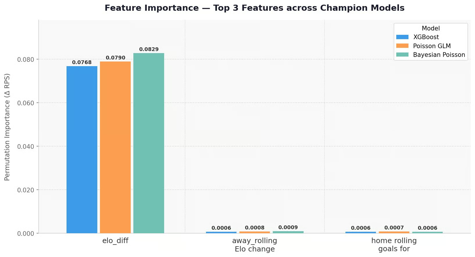
For the live tournament, I do not run all ten. I keep a smaller roster: the mean-rate baseline as a reference point, plus the three best performers. XGBoost and Bayesian Poisson take the top two spots outright.

Third place is effectively a tie: the Negative Binomial and Bivariate Poisson finish within 0.0002 RPS of each other and swap places depending on the random seed, so between two statistically indistinguishable models, I went with the Bivariate Poisson, whose formulation has the stronger footing in the football-prediction literature (Karlis and Ntzoufras, 2004).

That leaves a roster of XGBoost (machine learning), Bivariate Poisson (classical statistics), and Bayesian Poisson (Bayesian inference). The next section covers how those models run, retrain, and turn single-match predictions into a full tournament forecast.

Putting It Into Production

A model that lives in a notebook is only useful while you are sitting in front of it. To predict matches across a month-long tournament, the whole thing has to run on its own: pull new results, retrain, re-simulate, and refresh the forecast without anyone touching it. That is the job of the pipeline.

The bi-hourly pipeline on GCP

The entire project runs as a single scheduled job on Google Cloud Run. Before the tournament, it wakes up once a day; from the opening match on June 11, it runs every second hour. Each run follows the same cycle:

• Check for new data. If no matches have finished since the last run, there is nothing to do, and the job exits early.
• Ingest and rebuild. When new results have come in, they are pulled from the data sources, and a single dvc repro rebuilds the Silver and Gold layers so the features are current.
• Retrain, predict, simulate. The roster models are brought up to date (more on how in a moment), every upcoming matchup is predicted, and the full tournament is simulated.
• Score. Once a match is settled, the predictions made for it are scored, which feeds the monitoring described below.

Because every step is triggered by code on a schedule, there is no manual button-pressing during the tournament. New result in, refreshed forecast out.

Two modes: frozen vs. per-round

This is where the project doubles as an experiment. During the tournament, the roster runs in two parallel modes, and the difference between them is the question I hope to answer from the data: Does retraining as the tournament unfolds make the predictions better?

• Frozen. The models are locked the moment the tournament kicks off and never retrained. They still respond to results, because each simulation starts from the updated bracket, but the model parameters themselves never change.
• Per-round. The hyperparameters (the high-level settings) stay fixed, but the parameters the model learns are refitted on all available data after every completed group matchday and every knockout round, so the models keep learning from the tournament as it happens.

Running both side by side lets me compare them on two fronts once it is over: raw predictive accuracy, and how quickly each one's uncertainty resolves as the field narrows. If per-round wins, regular retraining earns its keep; if frozen holds its own, the extra machinery may not be worth it.

From predictions to a tournament: the Monte Carlo simulation

Predicting a single match is one thing. Turning that into "what is each team's chance of winning the tournament" is where the Monte Carlo simulation comes in.

First, inference. Rather than predicting only the fixtures we already know, the model predicts every possible matchup among the 48 teams. That sounds excessive, but in a tournament, any team could meet any other in the knockouts, so a prediction has to be ready for every pairing.

Next, the rules have to be encoded, and the 2026 format makes that especially awkward. Across the 12 groups, the top two advance automatically, but so do the eight best third-placed teams, and which knockout slot each of those eight lands in depends on which groups they came from.

There are 495 ways to choose eight qualifying groups out of twelve (twelve choose eight), and each one produces a different set of round-of-32 pairings. There is no clean formula for it; FIFA simply publishes a table. So I (or rather my very capable colleague Cursor) hardcoded all 495 combinations into a mapping, using the official table as the source.

"best_third_mappings": {
  "EFGHIJKL": {
    "74": "3F",
    "77": "3G",
    "79": "3E",
    "80": "3K",
    "81": "3I",
    "82": "3H",
    "85": "3J",
    "87": "3L"
  }, 
  "DFGHIJKL": ...

Each key, like EFGHIJKL, lists which eight groups supplied the advancing third-placed teams, and the values slot each of those teams (3E, 3F, and so on) into a specific round-of-32 match number. That is one entry; the full mapping repeats it 495 times, once per combination.

The three host nations (the United States, Canada, and Mexico) get one extra piece of handling. When a host plays a match staged in its own country, the simulation applies a home-advantage adjustment for that fixture, while the rest of the tournament is treated as neutral ground.

With the predictions and the rules in place, the simulation runs the whole tournament 10,000 times. In each run, it follows this procedure:

1. Draw a scoreline for every match by sampling home and away goals from the model's predicted distributions
2. Play out the group stage under the real points and tiebreak rules
3. Resolves the best-third table
4. Fills in the knockout bracket from the mappings above
5. Play through to a single champion.

Across 10,000 simulated tournaments, the share of runs in which a team reaches the final, or lifts the trophy, becomes that team's probability. One run is a guess; ten thousand runs is a forecast.

Tracking it all with MLflow

Every run described so far, in both modes, is logged to MLflow (hosted on DagsHub). Experiment tracking means systematically recording the inputs, settings, results, and outputs of each run, so any of them can be compared against the others or reproduced exactly. A few of the things it captures are worth calling out:

• Reproducibility. The simulation uses a fixed random seed derived from the tournament round, and the same seed is shared by the frozen and per-round modes. That means any difference between the two comes from the models themselves, not from the luck of the draw inside the simulation. Each run also logs the exact data snapshot it saw (the number of Gold rows and a timestamp), so results can always be traced back to their inputs.
• The experiment. Each run is tagged with its mode (frozen or per-round) and its stage in the lifecycle, from experimental and QA through to the live inference and refit runs, mirroring the promotion flow from the previous section.
• Comparison. Holdout RPS is logged as the selection metric, along with a reference to the current champion run for lineage. Fitting time is recorded as well, which is where the Bayesian model's roughly 100-times-slower training shows up in black and white.

The trained models and the prediction files themselves (the tournament probabilities, group standings, and match forecasts) are stored as run artifacts, and those files are exactly what the live dashboard reads. That closes the loop: from raw results, through training and simulation, to the numbers you can see online.

Monitoring for drift

The last piece runs once matches are settled. As real results arrive, the predictions made for them are scored and compared against the simple mean-rate baseline. If the full models start losing ground to a model that knows nothing about the teams, that is a warning sign of drift: the patterns learned before the tournament may no longer match what is happening on the pitch.

Watching for this is standard practice for any system making live predictions, and you can read more about how it is detected in this guide to data drift and model drift.

So, Who Wins the World Cup?

After all that machinery, here is what it is for.

The favorites

As of June 10, 2026, the day before the opening match, the model's verdict is clear at the very top and crowded just behind it. Spain and Argentina lead the field, each with roughly a 16% chance of lifting the trophy. That the reigning world champions (Argentina) and the reigning European champions (Spain) come out on top is a reassuring sanity check that the model is grounded in reality.

Behind them sits a tight chasing pack: France, England, Brazil, and Colombia round out the most likely winners. These are live figures, and they will move the moment real results start landing, so treat them as a June 10 snapshot rather than a fixed prophecy. The dashboard always shows the current numbers, with a maximum delay of two hours.

The live dashboard

Talking of which: Every number in this article comes from a live Streamlit app that updates automatically as the pipeline runs. You can open it at wc2026-predictions.streamlit.app and follow along through the tournament. It has four main views:

• Tournament overview: how far each team is expected to go, at a glance.
• Group standings: for every group, each team's probability of finishing first, second, third (split into third-and-through versus third-and-out, thanks to the best-third rule), or fourth.
• Match predictions: for each group game, the chance of a home win, draw, or away win, along with the most likely knockout bracket.
• Most common knockout matchups: the pairings the simulation produces most often.

One quirk worth flagging in the match view: a couple of teams appear in two possible round-of-32 slots at once. That is not a bug. It happens when a group is so evenly balanced that the model cannot confidently tell which qualifying position a team will take. Combined with the best-third uncertainty, the two outcomes lead to different knockout slots. In the case of Turkey, it even led to them being twice in the round of 16.

The following graphic shows the final rounds (quarterfinals until the final) that the XGBoost model projects before tournament kickoff:

The coin-flip team: United States

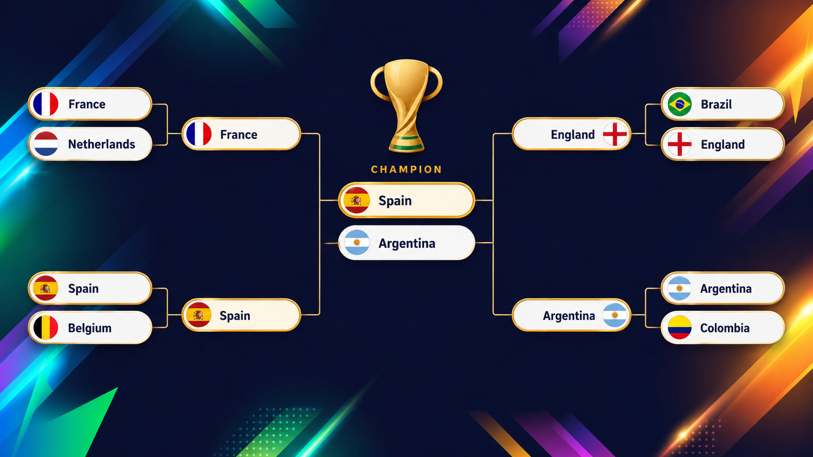
The fun of a model like this lies in the teams that defy the eye test, and the clearest example is the United States. If you go to the tournament overview on the dashboard, you will instantly notice that the US stands out in color.

As co-hosts playing in front of home crowds, you might expect a comfortable start, but the model is far more cautious: it gives them only about a 54.6% chance of escaping their group, the 13th-lowest in the entire field (remember that two-thirds of teams qualify for it!), because their group with Australia, Paraguay, and Turkey is unusually even.

The interesting part is what comes next. Having scraped through, the US then hovers at roughly a coin flip in every round that follows. Stack those coin flips together and they land at about a 2% chance of winning the whole tournament, which is the 13th-highest of all 48 teams.

A side that ranks 13th from the bottom to get out of its group and 13th from the top to win it all is just about the perfect definition of a coin-flip team: never the favorite, never out of it.

Final Thoughts

This project was a lot of work, and it covers far more ground than one article can hold. The repo has plenty that did not make it in here: the full set of candidate models, the feature engineering, and the orchestration that keeps everything running are some examples.

For now, the model has made its picks, and the tournament will be the judge. Whether you came for the MLOps or the football, I hope you enjoy watching it unfold as much as I will. You can follow the live forecast as the matches roll in and see how well the predictions hold up.

If you want to take a closer look at some of the concepts I mentioned, I recommend taking our MLOps Concepts course.